Polynomial Graphing Calculator

Welcome to Omni's polynomial graphing calculator, where we'll study how to graph polynomial functions. Obviously, the task gets more and more difficult when we raise the degree, and it becomes really complicated from five upwards. That's why we'll focus on polynomial function equations of degree at most four, where we're able to find the zeros of the polynomial, as well as its extrema and inflection points. Still, we'll also show a few universal tricks that you can apply to other cases, such as determining the end behavior of polynomial functions based on the leading coefficient of a polynomial.

By definition, polynomials are algebraic expressions in which variables appear only in non-negative integer powers. In other words, the letters cannot be, e.g., under roots, in the denominator of a rational expression, or inside a function. Let's see some polynomial function examples to get a grip on what we're talking about:

• $2x$;
• $(-3) \cdot z^3 \cdot 0.5$;
• $\pi r^2$;
• $x + 2y$;
• $a^2 + 2ab + b$: and
• $n^3 - 0.7n + (3/8)$.

Let us attract your attention to a few things here:

1. A polynomial can have several variables. In fact, it can even have none and still be called a polynomial (of degree zero).
2. The expression doesn't have to be in its simplest form. For instance, the product in the second expression above can surely be written in an easier way, yet we call both polynomials.
3. A polynomial's coefficients can be any real number. Note how above, we have integers, negative numbers, fractions, decimals, and even the $\pi$ from circle calculations.
4. Some polynomials have their special names. Those with only one expression (i.e., one summand) are monomials (e.g., the first three above). Those with two are binomials (e.g., the fourth above), and those with three are trinomials (e.g., the last two).
5. For polynomials with one variable, the coefficient next to the highest power of the variable is called the leading coefficient of the polynomial. It'll be crucial when studying the end behavior of polynomial functions in the next section.

Now that we know the terminology, it's time to get the crayons ready. Omni's polynomial graphing calculator focuses on expressions with one variable, which we denote $x$. We refer to the polynomial by $P(x)$ and treat it as a function of the variable.

In a moment, we'll see how to graph such polynomial functions on the two-dimensional Cartesian plane. The task requires finding the zeros of the polynomial as well as some of its most interesting points. It is in itself rather lengthy and difficult, but before we get to that, let's cover something simpler: the end behavior of polynomial functions.

In our case, "the end" refers to either minus or plus infinity. In other words, we wish to check what happens with our expressions when the variable $x$ is extremely small (as a negative number) or extremely large.

For instance, take two polynomial function equations: $P(x) = x^2$ and $R(x) = x^3$. Let's see how their values change for several instances of $x$.

We see that $P(x)$ and $R(x)$ both rise quickly for large (positive) $x$. On the other hand, if we go with $x$ the other way, i.e., make it negative, then $P(x)$ increases but $R(x)$ decreases. We can easily imagine that the trend continues for values beyond the ones in the table above.

All in all, we can describe the end behavior of the polynomial functions as follows:

• When $x$ goes towards plus infinity:
  • $P(x)$ goes to plus infinity; and
  • $R(x)$ goes to plus infinity.
• When $x$ goes towards minus infinity:
  • $P(x)$ goes to plus infinity; and
  • $R(x)$ goes to minus infinity.

It's easy to see that the thing depended only on the parity of the exponent: the squared function killed the minus, while the cubed one didn't. Furthermore, observe how the signs would flip if we had $S(x) = -x^2$ and $T(x) = -x^3$ instead.

In fact, even for more complicated expressions such as, say, $x^2 - 17x - 89$, it boils down to the single summand with the highest power of $x$. That is because the highest exponent dominates over any lower ones for extreme values. Therefore, we only need to check what is called the leading coefficient of the polynomial. However, note how it doesn't really matter if it's $2x^2$ or $361x^2$: the function will still go to plus infinity, though slightly faster in the second case.

To sum it all up, let's have a neat instruction on how to determine the end behavior of polynomial functions based on the leading coefficient of the polynomial.

If the highest exponent of a polynomial is:

• Even and the leading coefficient is:
  • Positive, then the function goes to:
    • Plus infinity for $x$ going to plus infinity; and
    • Plus infinity for $x$ going to minus infinity.
  • Negative, then the function goes to:
    • Minus infinity for $x$ going to plus infinity; and
    • Minus infinity for $x$ going to minus infinity.
• Odd and the leading coefficient is:
  • Positive, then the function goes to:
    • Plus infinity for $x$ going to plus infinity; and
    • minus infinity for $x$ going to minus infinity.
  • Negative, then the function goes to:
    • Minus infinity for $x$ going to plus infinity; and
    • Plus infinity for $x$ going to minus infinity.

Alright, we've figured out how to graph polynomial functions, or at least, their ends. Let's now see how to deal with everything that happens in between.

A zero of a polynomial (also called its root; not to be confused with radicals) is a point where the function is equal to zero. For example, $P(x) = x^2 - 2x + 1$ has a zero in $x = 1$ since:

For linear equations (i.e., polynomials of degree $1$), finding their root is simple: it boils down to a couple of arithmetic operations. For quadratic ones, we have some nice formulas that use the discriminant, so it's not too bad. Still, this time, there may be two, one, or zero solutions, so the matter is a bit more complicated.

In fact, there are formulas for polynomials of degree $3$ and $4$ too. However, this time the word "complicated" doesn't really touch the surface: they are extremely long, require tedious work, and, as before, there may be different numbers of solutions for various polynomial function examples. If you're interested, make sure to read more about cubic functions and quartic functions.

Either way, finding the zeros of a polynomial is often the first step when drawing the function on the Cartesian plane. For a given $P(x)$, this means solving the associated polynomial function equation: $P(x) = 0$. The solutions are the zeros, i.e., the points where the graph of $P(x)$ touches the horizontal line.

Next, we look for the critical points of the function. While the roots told us where the graph meets the horizontal line, these new points describe what happens in between: if the values increase or decrease and until what number.

By definition, a critical point of a polynomial is a value $x_0$ where the derivative vanishes. Therefore, for a given $P(x)$, we need to solve the equation $P'(x) = 0$ to get the zeros of the derivative, i.e., the critical points of $P(x)$. Recall that for:

we have:

Observe that the degree of the derivative is always $1$ smaller than that of the initial polynomial. As such, finding the critical points of, e.g., a cubic equation requires solving a quadratic equation.

We distinguish two types of critical points: extrema and inflection points.

1. Extrema

   Or, more precisely, local extrema. They are points where the polynomial (not the derivative, mind you!) attains extreme values. To be precise, around that point (or, as mathematicians call it, in its neighborhood), all other values are smaller (which means it's a maximum) or larger (which means it's a minimum): believe it or not but we have a calculator for this too, the minimum and maximum calculator!

   The best example of a polynomial function's extremum is the vertex of a parabola — you can learn how to calculate it here, at the parabola calculator. For instance, draw the functions $P(x) = x^2$ and $R(x) = -x^2$. Both of them have their vertices in point $(0,0)$, but they are, respectively, the local minimum (since all other values of $P(x)$ are larger than $0$) and local maximum (since all other values of $R(x)$ are smaller than $0$).

2. Inflection points

   These are points that wanted to be extrema, but mom didn't let them.

   Recall the two polynomial function examples from point 1. above: $P(x) = x^2$ and $R(x) = -x^2$. In both cases, the graphs flatten when they approach the point $x = 0$ from either side and when they pass $0$, they change their course.

   When a graph approaches its inflection point, it also flattens. However, in this case, it doesn't change the course once it passes. Instead, it repeats what it has been doing: decreases if it has been decreasing or increases if it has been increasing.

   As an example, consider the polynomial function equations $S(x) = x^3$ and $T(x) = -x^3$. Both of them flatten when they approach the point $x = 0$ from either side and continue the previous pattern when they pass it. Note how in point 1., we distinguished between the two examples and had minima or maxima. Here, on the other hand, we call both instances simply inflection points.

Note how Omni's polynomial graphing calculator automatically calculates the functions roots, critical points, extrema, and inflection points. We encourage you to seek the values on the graph provided by the tool to see how they affect the function. In fact, let us do just that on a simple example and take the opportunity to present the functionalities of the polynomial graphing calculator.

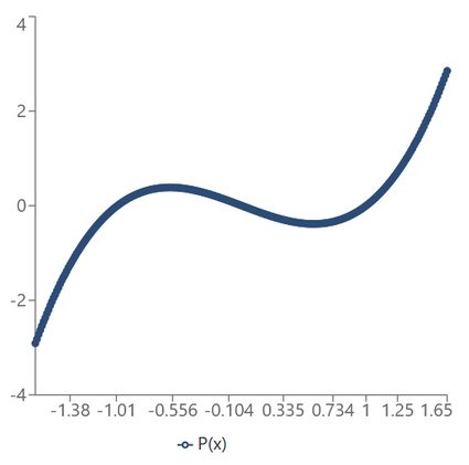
Let's see how to graph the polynomial function $P(x) = x^3 - x$.

First of all, we use Omni's polynomial graphing calculator to do the work for us. There, we begin by telling what type of a function we have. In our case, it's a cubic polynomial, so we choose $3$ under "Polynomial degree." That'll show a symbolic representation of such an expression underneath and corresponding variable fields farther down. Looking back at our polynomial function example, we input:

Note how we have $a₂ = 0$ and $a₀ = 0$ since $P(x)$ has no terms with $x^2$ or with no $x$ at all. Also, we input $a_3 = 1$ and $a_1 = -1$ even though there are no numbers in the corresponding places in $P(x)$. That's because, by convention, we don't write $1$-s in front of variables. However, observe that we needed to remember about the minus in $a_1$.

The moment we input the last coefficient, Omni's polynomial graphing calculator will draw the graph, as well as find the zeros of the polynomial together with its critical points, extrema, and inflection points. Let us also mention that in case you'd like to see some other section of the graph than the one presented, you may go into the advanced mode and input a custom interval.

Now let's try to describe the graph ourselves. First of all, we need to find the zeros of the polynomial, so we solve the equation $P(x) = 0$:

We obtained a product which is equal to $0$, which means one of its factors must be zero. In other words, we have $x = 0$, $x - 1 = 0$, or $x + 1 = 0$, which gives us three solutions: $x = 0$, $x = 1$, and $x = -1$.

Next, we look for critical points. For that, we compute the derivative $P'(x)$ according to the formula from the above section:

Now, we solve the equation $P'(x) = 0$:

which gives us two solutions (i.e., critical points): $-\sqrt{3}/3\approx -0.577$ and $\sqrt{3}/3\approx 0.577$.

Lastly, we draw the graph. Note that the leading coefficient of the polynomial is positive (i.e., equal to $1$), and it's in front of an odd power of $x$ (i.e., $x^3$). That means the end behavior of the polynomial function is as follows:

• $P(x)$ goes to plus infinity when $x$ goes to plus infinity; and
• $P(x)$ goes to minus infinity when $x$ goes to minus infinity.

In between, the graph must touch the vertical axis in points $-1$, $0$, and $1$, and flatten in $-0.577$ and $0.577$. That takes us to the conclusion that $P(x)$ has a local maximum in $x = -0.577$ and a local minimum in $x = 0.577$; it has no inflection points.

All in all, the graph of $P(x) = x^3 - x$ looks like this:

Make sure to experiment with the polynomial graphing calculator to see how different coefficients affect the zeros and the bumps.

To graph polynomial functions, say, P(x), you need to:

1. Solve the equation P(x) = 0 to find the zeros of P(x).

2. Determine the end behavior by checking the leading coefficient.

3. Compute the derivative P'(x).

4. Solve the equation P'(x) = 0 to find the critical points of P(x).

5. Evaluate the polynomial in all the critical points.

6. For each point in 4., check if it's an extremum or an inflection point.

7. Draw the actual graph:

   • Mark all the zeros and critical points.
   • Draw the ends according to point 2.
   • Graph the polynomial in between by:
     • Starting from the right end.
     • Touching the vertical axis in the zeros.
     • Reflecting the line in the extrema.
     • Passing through the inflection points.

To determine the end behavior of a polynomial function in x, you need to:

1. Find the parity of the highest variable power in the polynomial.
2. Determine its coefficient: is it positive or negative?
3. If the exponent is:
   • Even, then:
     • For a positive leading coefficient, the function tends to:
       • +∞ for x approaching +∞; and
       • +∞ for x approaching -∞.
     • For a negative leading coefficient, the function tends to:
       • -∞ for x approaching +∞; and
       • -∞ for x approaching -∞.
   • Odd, then:
     • For a positive leading coefficient, the function tends to:
       • +∞ for x approaching +∞; and
       • -∞ for x approaching -∞.
     • For a negative leading coefficient, the function tends to:
       • -∞ for x approaching +∞; and
       • +∞ for x approaching -∞.

To draw the graph of a quadratic polynomial P(x) = ax² + bx + c, you need to:

1. Find the real solutions to P(x) = 0 (i.e., the zeros).
2. Solve the derivative equation 2ax + b = 0.
3. Evaluate P(x) in the point obtained in 2.
4. Mark the values from points 1-2. on the vertical axis.
5. Mark the parabola's vertex given by points 2-3.
6. Draw the actual graph:
   • Start from the vertex and draw the arms:
     • Upwards if a > 0; or
     • Downwards if a < 0.
   • Make sure the arms cross the vertical axis in the zeros (if there are any).

To analyze graphs of polynomial functions, make sure to check where the graph:

• Touches the vertical axis (those are the polynomial's zeros);
• Tends to on the far-left and far right (those describe the end behavior);
• Has bumps (those are the function's extrema); and
• Flattens, but then continues increasing/decreasing (those are the inflection points).

The degree of a polynomial affects the graph in the following ways:

• The degree's parity determines the end behavior: whether it's the same on both ends or not;
• The number of zeros: the graph may touch the vertical axis at most as many times as given by the degree; and
• The number of critical points: the number of extrema and inflection points is, at most, one smaller than the degree.

To draw the graph of a cubic polynomial P(x) = ax³ + bx² + cx + d, you need to:

1. Find the real solutions to P(x) = 0.
2. Solve the derivative equation 3ax² + 2bx + c = 0.
3. Evaluate P(x) in the points obtained in 2. (if there are any).
4. Mark the values from points 1-2. on the vertical axis.
5. Mark the critical points given by points 2-3. (if there are any).
6. Draw the actual graph:
   • Start from:
     • The upper right if a > 0; or
     • The bottom right if a < 0.
   • Make sure to touch the vertical line in all the points from 1.
   • If in point 2. you got:
     • Two values reflect the graph in points from 5. (they are extrema);
     • One value, go through the point from 5. and continue increasing/decreasing (it's an inflection point); or
     • No values, do none of the above.
   • Make sure to finish the graph on:
     • The bottom left if a > 0; or
     • The upper left if a < 0.