Cramer's Rule Calculator

Welcome to the Cramer's rule calculator, a quick and easy 2- and 3-variable system of equations solver. Together, we'll learn how to construct a coefficient matrix and then try using those matrices to solve systems of equations. You might have already seen one or two different ways to tackle similar mathematical problems. However, we're here to convince you that Cramer's rule for 3x3 matrices is almost as easy as Cramer's rule for 2x2 matrices (which is super easy)!

So, would you like to learn how to solve systems of equations with a matrix or two, without any substitution, elimination, or drawing graphs - just simple arithmetics?

You know how not everything in life is known, or easy to describe? Like how fast does the universe expand, how much can you save on Black Friday, or how many apples did Mr. Smith buy if he paid $3.50 and one costs $0.50? You know, the essential questions in life.

Whenever we don't know some number explicitly, but we can describe it in relation to some other numbers, we obtain an equation. Mathematically speaking, it's a symbolic description of an equality that our value must satisfy. For example, we can write the third question as follows:

$\text {cost of one apple} × \$0.50 = \$3.50$.

The $\text {cost of one apple}$ is the value that we don't know and would like to find. Usually, we call such a thing a variable and denote it by a single letter, say, $\text x$. The equation above then looks like this:

$\text x × \$0.50 = \$3.50$.

That's a pretty simple one, and we can easily calculate that Mr. Smith bought seven apples. However, life is not always that easy. Not only can Mr. Smith buy more apples, but he can also, for example, give a tip to the shopkeeper. We would then have to include that in the equation we construct, which would make it a little more complicated. But what if Mr. Smith wants to buy some oranges as well?

If a new value enters the picture and we don't know it either, we must introduce it as a new variable, say $\text y$. When we describe our two variable question, what we get is still an equation, however, in general, they become more difficult to calculate.

Nevertheless, if we have more information, the problem looks much more promising. For instance, if on one occasion Mr. Smith bought 7 apples and 3 oranges and paid $5.60, and on another he bought 1 apple and 5 oranges, and paid $4.00, then this is enough information to calculate how much an apple and an orange cost. This is because we can write two equations (one for each shopping) with two variables. We call such a thing a system of equations.

To sum up, in general, a system of equations is a number of equations with a few variables, and we want to find numbers that satisfy all of these equations. We will now describe how to solve such a system of equations with a matrix.

How about checking out our matrix multiplication calculator to learn about an interesting concept on matrices.

Let's look at a traveling-themed problem:

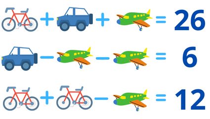
At first, it may not look like a system of equations, but in fact, it is just that. After all, the $\text x$'s and $\text y$'s we used in the section above are just examples of how we can denote a variable; there is no reason why we can't use bikes instead.

However, for simplicity of notation, and for the sake of our 3-variable system of equations solver, let's switch to the boring mathematical notation, and say that $\text x$ will denote the bike, $\text y$ the car, and $\text z$ the plane. Then we can write the above system as

$\text x + \text y + \text z = 26$;

$\text y - \text z - \text z = 6$; and

$\text x + \text x - \text z = 12$.

We have three equations and three variables, so our end-goal is to use Cramer's rule for 3x3 matrices (the first 3 denote the number of equations, the second the number of variables). To do this, we first need to construct an array of numbers, which we'll call the coefficient matrix.

Before that, however, we have to work a little to make our system more like the one we see in our Cramer's rule calculator. Note that we can simplify the two last equations, i.e., add together the same variables in each line. For example, in the bottom equation, we have $\text x + \text x$, which we can write as $2\text x$ (one copy of $\text x$ plus one copy of $\text x$ equals two copies of $\text x$). All in all, we obtain

$\text x + \text y + \text z = 26$

$\text y - 2 \text z = 6$

$2\text x - \text z = 12$.

Now we're ready to form the coefficient matrix. It will be an array with three rows (because we have three equations) and three columns (because we have three coefficients). The first column will correspond to the variable $\text x$, the second to $\text y$, and the third to $\text z$. Here, by "correspond," we mean that it will contain the coefficients of that variable in consecutive equations (hence the name coefficient matrix). Note, that we don't have all the variables in all the lines. For example, the second equation doesn't have the $\text x$ variable. Fortunately, this simply means that the coefficient of $\text x$ in that line is, in fact, zero.

To sum up, the number in row $\text i$ and column $\text j$ in the coefficient matrix contains the number next to $\text j$-th coefficient (the first being $\text x$, the second $\text y$, and the third $\text z$) in the $\text i$-th equation. In our case, it will look as follows:

Quite often, it is useful to define the so-called augmented coefficient matrix. It is the same thing with an additional column to the right, with the right-hand side numbers of the equalities of our system. Usually, it is separated from the others by a dashed line. In our case, it looks like this:

Let's not waste a minute more and start using these matrices to solve systems of equations using Cramer's rule for 3x3 systems.

Most of the ways of dealing with systems of equations is to change the system itself a lot - reducing its rows, substituting one value for another, and so on. It tends to get messy in more complicated examples. Cramer's rule is a way to hide all of that with a few simple arithmetic operations on the coefficient matrix, namely calculating a few determinants.

The determinant of a square matrix is a number that we get from multiplying and adding some of the cells of the matrix. Since our Cramer's rule calculator is a 2- and 3-variable system of equations solver, we'll focus on the formulas for when we have two equations with two variables and three equations with three variables.

If

then the determinant of $\text A$, denoted $|\text A|$ or $\text {det(A)}$, is

$|\text A| = \text {a×d} - \text {b×c}$.

And if

then the determinant of $B$ is

$|\text B| =\text {a×e×i} + \text {b×f×g} + \text {c×d×h} - \text {c×e×g} - \text {b×d×i} - \text {a×f×h}$

Now denote the coefficient matrix of our system by $W$ (note that it is a 2x2 matrix when we have two equations and two variables, and 3x3 when we have three equations and three variables). We will now define some additional matrices, $\text W_\text x$, $\text W_\text y$, and $\text W_\text z$, that will correspond to each variable of our system ($\text W_\text z$ exists only when we have $\text z$ in the equations).

You may want to try out our eigenvalue and eigenvector calculator.

Recall the augmented coefficient matrix from the section above. It had an additional column with the numbers on the right hand side of the $=$ sign in the system. We define the matrices corresponding to variables to be the initial coefficient matrix with the column of the variable in question swapped for the extra, right hand side column. For instance, the matrix $\text W_\text z$ will have the same first two columns (corresponding to $\text x$ and $\text y$) as $\text W$, while its third column will be the additional one from the augmented coefficient matrix.

The Cramer's rule for 2x2 systems states that the system's solution is given by

$\text x = |\text W_\text x| / |\text W|$

$\text y = |\text W_\text y| / |\text W|$

and the Cramer's rule for 3x3 systems adds to that a third variable:

$\text z = |\text W_\text z| / |\text W|$

Note, that when we use these formulas to solve a system of equations, each matrix mentioned above is 2x2 in size when we have two equations and two variables, and 3x3 in size when we have three equations and three variables.

Things to remember:

• Using matrices to solve systems of equations with Cramer's rule allows us to find the answer by simply following a few predetermined calculations. There is almost no thinking here, only multiplication, addition, and division;
• We can use the above description as a step-by-step 2- and 3-variable system of equations solver. However, Cramer's rule still applies to larger matrices, although the calculations can get a little messy. In particular, the determinant gets pretty ugly. The number of summands in the formula is equal to the number of permutations. This means that for four equations with four variables, it has 24, and for five, it has 120 summands;
• The determinant of a matrix can be zero. If it's the $\text W$ matrix, then we have a problem: we cannot divide by zero! This can mean two things: either we have no solutions, or we have infinitely many of them. The first case is when at least one of the variable matrices is non-zero, and the latter when all of them are zero (together with $\text W$);
• Our Cramer's rule calculator will tell you if we're dealing with one of the two special cases we've mentioned above. Even better, if there are infinitely many solutions, it will also describe the form of the pairs/triples that satisfy the system; and
• Try to get a decent amount of sleep every day. It's always good to remember that.

Recall the traveling-based example from section two and the system of equations that we got from it after simplifying each line:

$\text {x + y + z} = 26$;

$\text y - 2\text z = 6$; and

$2\text x - \text z = 12$.

Let's also remind ourselves of the augmented coefficient matrix:

Before we move on to construct the four matrices used in Cramer's rule for 3x3 systems, let's take some time to describe how we can input the data into the Cramer's rule calculator.

We have three equations to deal with, so let's tell the calculator that by choosing the right option in the "Number of equations" field. This will turn our tool into a 3-variable system of equations solver and show us a picture of what such a system looks like, with a few mysterious symbols, like $\text a_1$ or $\text c_2$. These denote the coefficients of our system, i.e., the numbers that stand to the left of the variables in each line and the numbers to the right of the $=$ sign.

This notation is listed in the calculator, where you can input the values from the problem that you want to solve. The $\text a$'s correspond to the numbers next to $\text x$'s, the $\text b$'s to $\text y$'s, the $\text c$'s to $\text z$'s, the $\text d$'s are the numbers on the right, and the indices tell us the number of the row. Note that our Cramer's rule calculator accepts only linear equations. This means that we cannot, for example, have a quadratic one, or an expression with a variable under a square root.

Observe that those coefficients are also in our augmented coefficient matrix. In fact, it is enough to copy them into the Cramer's rule calculator. For example, the first row of the matrix has numbers $1$, $1$, $1$, and $26$. It corresponds to the first equation, which has coefficients denoted with the subscript $₁$. Therefore, we have:

$\text a_1 = 1$, $\text b_1 = 1$, $\text c_1 = 1$, $\text d_1 = 26$.

Similarly, the other two rows give us:

$\text a_2 = 0$, $\text b_2 = 1$, $\text c_2 = -2$, $\text d_2 = 6$; and

$\text a_3 = 2$, $\text b_3 = 0$, $\text c_3 = -1$, $\text d_3 = 12$.

Once you get all that data into the Cramer's rule calculator, it should spit out the values of the four determinants, followed by the solution to the system. Let's look how it figured that out.

As we've mentioned in the section above, Cramer's rule for 2x2 and 3x3 systems means that we have to calculate the determinants of a few matrices. The first one, the so-called main one, is simply the coefficient matrix that we've defined in section two:

To construct the other three, we'll need to exchange one column of this matrix with the fourth extra column of the augmented coefficient matrix, which in our case has numbers $26$, $6$, and $12$. To get $\text W_\text x$, the $\text x$ matrix, we put those numbers instead of the column corresponding to the $\text x$ variable, namely the first one:

Similarly, we get

All we need to do is use the determinant formula from the section above for all four of the matrices:

$|\text W| = 1\times 1 \times (-1) + 1\times (-2)\times 2 + 1\times 0\times 0 - 1\times 1\times 2 - 1\times 0\times (-1) - 1\times (-2)\times 0 = -7$

$|\text W_\text x| = 26\times 1\times (-1) + 1\times (-2)\times 12 + 1\times 6\times 0 - 1\times 1\times 26 - 1\times 6\times (-1) - 26\times (-2)\times 0 = -56$

$|\text W_\text y| = 1\times 26\times (-1) + 26\times (-2)\times 2 + 1\times 0\times 12 - 1\times 6\times 2 - 26\times 0\times (-1) - 1\times (-2)\times 12 = -98$

$|\text W_\text z| = 1\times 1\times 12 + 1\times 6\times 2 + 26\times 0\times 0 - 26\times 1\times 2 - 1\times 0\times 12 - 1\times 6\times 0 = -28$.

Lastly, we use Cramer's rule for 3x3 systems and obtain the solution:

$\text x = |\text W_\text x| / |\text W| = -56 / (-7) = 8$,

$\text y = |\text W_\text y| / |\text W| = -98 / (-7) = 14$,

$\text z = |\text W_\text z| / |\text W| = -28 / (-7) = 4$.

Going back to the problem we started with, this means that the bike is equal to $8$, the car is equal to $14$, and the plane is equal to $4$.

We have a tool called reduced row echelon form calculator, where we solve a system of equations of your choice using the matrix row reduction and elementary row operations.