Z-test Calculator

This Z-test calculator is a tool that helps you perform a one-sample Z-test on the population's mean. Two forms of this test - a two-tailed Z-test and a one-tailed Z-tests - exist, and can be used depending on your needs. You can also choose whether the calculator should determine the p-value from Z-test or you'd rather use the critical value approach!

Read on to learn more about Z-test in statistics, and, in particular, when to use Z-tests, what is the Z-test formula, and whether to use Z-test vs. t-test. As a bonus, we give some step-by-step examples of how to perform Z-tests!

Or you may also check our t-statistic calculator, where you can learn the concept of another essential statistic. If you are also interested in F-test, check our F-statistic calculator.

A one sample Z-test is one of the most popular location tests. The null hypothesis is that the population mean value is equal to a given number, $\mu_0$:

We perform a two-tailed Z-test if we want to test whether the population mean is not $\mu_0$:

and a one-tailed Z-test if we want to test whether the population mean is less/greater than $\mu_0$:

Let us now discuss the assumptions of a one-sample Z-test.

You may use a Z-test if your sample consists of independent data points and:

• the data is normally distributed, and you know the population variance;

  or

• the sample is large, and data follows a distribution which has a finite mean and variance. You don't need to know the population variance.

The reason these two possibilities exist is that we want the test statistics that follow the standard normal distribution $\mathrm N(0, 1)$. In the former case, it is an exact standard normal distribution, while in the latter, it is approximately so, thanks to the central limit theorem.

The question remains, "When is my sample considered large?" Well, there's no universal criterion. In general, the more data points you have, the better the approximation works. Statistics textbooks recommend having no fewer than 50 data points, while 30 is considered the bare minimum.

Let $x_1, ..., x_n$ be an independent sample following the normal distribution $\mathrm N(\mu, \sigma^2)$, i.e., with a mean equal to $\mu$, and variance equal to $\sigma ^2$.

We pose the null hypothesis, $\mathrm H_0 \!\!:\!\! \mu = \mu_0$.

We define the test statistic, Z, as:

where:

• $\bar x$ is the sample mean, i.e., $\bar x = (x_1 + ... + x_n) / n$;

• $\mu_0$ is the mean postulated in $\mathrm H_0$;

• $n$ is sample size; and

• $\sigma$ is the population standard deviation.

In what follows, the uppercase $Z$ stands for the test statistic (treated as a random variable), while the lowercase $z$ will denote an actual value of $Z$, computed for a given sample drawn from N(μ,σ²).

If $\mathrm H_0$ holds, then the sum $S_n = x_1 + ... + x_n$ follows the normal distribution, with mean $n \mu_0$ and variance $n^2 \sigma$. As $Z$ is the standardization (z-score) of $S_n/n$, we can conclude that the test statistic $Z$ follows the standard normal distribution $\mathrm N(0, 1)$, provided that $\mathrm H_0$ is true. By the way, we have the z-score calculator if you want to focus on this value alone.

If our data does not follow a normal distribution, or if the population standard deviation is unknown (and thus in the formula for $Z$ we substitute the population standard deviation $\sigma$ with sample standard deviation), then the test statistics $Z$ is not necessarily normal. However, if the sample is sufficiently large, then the central limit theorem guarantees that $Z$ is approximately $\mathrm N(0, 1)$.

In the sections below, we will explain to you how to use the value of the test statistic, $z$, to make a decision, whether or not you should reject the null hypothesis. Two approaches can be used in order to arrive at that decision: the p-value approach, and critical value approach - and we cover both of them! Which one should you use? In the past, the critical value approach was more popular because it was difficult to calculate p-value from Z-test. However, with help of modern computers, we can do it fairly easily, and with decent precision. In general, you are strongly advised to report the p-value of your tests!

Formally, the p-value is the smallest level of significance at which the null hypothesis could be rejected. More intuitively, p-value answers the questions:
provided that I live in a world where the null hypothesis holds, how probable is it that the value of the test statistic will be at least as extreme as the $z$-value I've got for my sample? Hence, a small p-value means that your result is very improbable under the null hypothesis, and so there is strong evidence against the null hypothesis - the smaller the p-value, the stronger the evidence.

To find the p-value, you have to calculate the probability that the test statistic, $Z$, is at least as extreme as the value we've actually observed, $z$, provided that the null hypothesis is true. (The probability of an event calculated under the assumption that $\mathrm H_0$ is true will be denoted as $\small \mathrm{Pr}(\text{event} | \mathrm{H_0})$.) It is the alternative hypothesis which determines what more extreme means:

1. Two-tailed Z-test: extreme values are those whose absolute value exceeds $|z|$, so those smaller than $-|z|$ or greater than $|z|$. Therefore, we have:

The symmetry of the normal distribution gives:

2. Left-tailed Z-test: extreme values are those smaller than $z$, so

3. Right-tailed Z-test: extreme values are those greater than $z$, so

To compute these probabilities, we can use the cumulative distribution function, (cdf) of $\mathrm N(0, 1)$, which for a real number, $x$, is defined as:

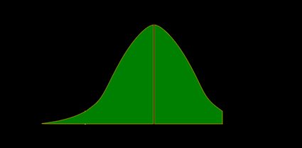
Also, p-values can be nicely depicted as the area under the probability density function (pdf) of $\mathrm N(0, 1)$, due to:

With all the knowledge you've got from the previous section, you're ready to learn about Z-tests.

1. Two-tailed Z-test:

From the fact that $\Phi(-z) = 1 - \Phi(z)$, we deduce that

The p-value is the area under the probability distribution function (pdf) both to the left of $-|z|$, and to the right of $|z|$:

2. Left-tailed Z-test:

The p-value is the area under the pdf to the left of our $z$:

3. Right-tailed Z-test:

The p-value is the area under the pdf to the right of $z$:

The decision as to whether or not you should reject the null hypothesis can be now made at any significance level, $\alpha$, you desire!

• if the p-value is less than, or equal to, $\alpha$, the null hypothesis is rejected at this significance level; and

• if the p-value is greater than $\alpha$, then there is not enough evidence to reject the null hypothesis at this significance level.

The critical value approach involves comparing the value of the test statistic obtained for our sample, $z$, to the so-called critical values. These values constitute the boundaries of regions where the test statistic is highly improbable to lie. Those regions are often referred to as the critical regions, or rejection regions. The decision of whether or not you should reject the null hypothesis is then based on whether or not our $z$ belongs to the critical region.

The critical regions depend on a significance level, $\alpha$, of the test, and on the alternative hypothesis. The choice of $\alpha$ is arbitrary; in practice, the values of 0.1, 0.05, or 0.01 are most commonly used as $\alpha$.

Once we agree on the value of $\alpha$, we can easily determine the critical regions of the Z-test:

1. Two-tailed Z-test:

2. Left-tailed Z-test:

3. Right-tailed Z-test:

To decide the fate of $\mathrm H_0$, check whether or not your $z$ falls in the critical region:

• If yes, then reject $\mathrm H_0$ and accept $\mathrm H_1$; and

• If no, then there is not enough evidence to reject $\mathrm H_0$.

As you see, the formulae for the critical values of Z-tests involve the inverse, $\Phi^{-1}$, of the cumulative distribution function (cdf) of $\mathrm N(0, 1)$.

Our calculator reduces all the complicated steps:

1. Choose the alternative hypothesis: two-tailed or left/right-tailed.

2. In our Z-test calculator, you can decide whether to use the p-value or critical regions approach. In the latter case, set the significance level, $\alpha$.

3. Enter the value of the test statistic, $z$. If you don't know it, then you can enter some data that will allow us to calculate your $z$ for you:

   • sample mean $\bar x$ (If you have raw data, go to the average calculator to determine the mean);
   • tested mean $\mu_0$;
   • sample size $n$; and
   • population standard deviation $\sigma$ (or sample standard deviation if your sample is large).

4. Results appear immediately below the calculator.

If you want to find $z$ based on p-value, please remember that in the case of two-tailed tests there are two possible values of $z$: one positive and one negative, and they are opposite numbers. This Z-test calculator returns the positive value in such a case. In order to find the other possible value of $z$ for a given p-value, just take the number opposite to the value of $z$ displayed by the calculator.

To make sure that you've fully understood the essence of Z-test, let's go through some examples:

1. A bottle filling machine follows a normal distribution. Its standard deviation, as declared by the manufacturer, is equal to 30 ml. A juice seller claims that the volume poured in each bottle is, on average, one liter, i.e., 1000 ml, but we suspect that in fact the average volume is smaller than that...

Formally, the hypotheses that we set are the following:

• $\mathrm H_0 \! : \mu = 1000 \text{ ml}$

• $\mathrm H_1 \! : \mu \lt 1000 \text{ ml}$

We went to a shop and bought a sample of 9 bottles. After carefully measuring the volume of juice in each bottle, we've obtained the following sample (in milliliters):

$\small 1020, 970, 1000, 980, 1010, 930, 950, 980, 980$.

• Sample size: $n = 9$;

• Sample mean: $\bar x = 980 \ \mathrm{ml}$;

• Population standard deviation: $\sigma = 30 \ \mathrm{ml}$;

• So

• And, therefore, $\text{p-value} = \Phi(-2) \approx 0.0228$.

  As $0.0228 \lt 0.05$, we conclude that our suspicions aren't groundless; at the most common significance level, 0.05, we would reject the producer's claim, $\mathrm H_0$, and accept the alternative hypothesis, $\mathrm H_1$.

2. We tossed a coin 50 times. We got 20 tails and 30 heads. Is there sufficient evidence to claim that the coin is biased?

   Clearly, our data follows Bernoulli distribution, with some success probability $p$ and variance $\sigma^2 = p (1-p)$. However, the sample is large, so we can safely perform a Z-test. We adopt the convention that getting tails is a success.

   Let us state the null and alternative hypotheses:

   • $\mathrm H_0 \! : p = 0.5$ (the coin is fair - the probability of tails is $0.5$)

   • $\mathrm H_1 \! : p \ne 0.5$ (the coin is biased - the probability of tails differs from $0.5$)

In our sample we have 20 successes (denoted by ones) and 30 failures (denoted by zeros), so:

• Sample size $n = 50$;

• Sample mean $\bar x = 20/50 = 0.4$;

• Population standard deviation is given by $\sigma = \sqrt{0.5 \times 0.5}$ (because $0.5$ is the proportion $p$ hypothesized in $\mathrm H_0$). Hence, $\sigma = 0.5$;

• So

• And, therefore

Since $0.1573 \gt 0.1$ we don't have enough evidence to reject the claim that the coin is fair, even at such a large significance level as $0.1$. In that case, you may safely toss it to your Witcher or use the coin flip probability calculator to find your chances of getting, e.g., 10 heads in a row (which are extremely low!).

We use a t-test for testing the population mean of a normally distributed dataset which had an unknown population standard deviation. We get this by replacing the population standard deviation in the Z-test statistic formula by the sample standard deviation, which means that this new test statistic follows (provided that H₀ holds) the t-Student distribution with n-1 degrees of freedom instead of N(0,1).

For large samples, the t-Student distribution with n degrees of freedom approaches the N(0,1). Hence, as long as there are a sufficient number of data points (at least 30), it does not really matter whether you use the Z-test or the t-test, since the results will be almost identical. However, for small samples with unknown variance, remember to use the t-test instead of Z-test.

To calculate the Z test statistic:

1. Compute the arithmetic mean of your sample.
2. From this mean subtract the mean postulated in null hypothesis.
3. Multiply by the square root of size sample.
4. Divide by the population standard deviation.
5. That's it, you've just computed the Z test statistic!