Poisson Distribution Calculator

If you want to know the probability of an event happening a number of times over some interval, this Poisson distribution calculator is your go-to tool. Read on to find out what kinds of events are suitable for analysis using this calculator, and what is the Poisson distribution formula. We will present some Poisson distribution examples, too.

The Poisson distribution is a probability distribution (such as, for instance, the binomial distribution). It describes the probability of a certain number of events occurring during some time period. For the most part, you may use past data to determine this probability and learn about the frequency of events.

For example, suppose we know that the typical number of tornadoes a specific region experiences over ten years is 5. In that case, we can calculate the probability of no tornadoes troubling this area during the next ten year period. We can also find the probability of any other number of tornadoes appearing there during the next ten years.

Some examples of events that can be analyzed with the Poisson distribution calculator include:

• Number of buses arriving at a bus stop per hour;
• Number of blurred photos in a sample of 1,000 pictures taken with a camera;
• Number of meteors hitting the Earth over 100 years;
• Number of times a student is absent from class during the school year; and
• Number of visitors in a museum between 10 am and 11 am.

As you can see, the Poisson distribution is a convenient way of characterizing events that are independent of each other, and their probability does not vary over time. You can think about such events as accidents that happen at random, but sooner or later, they inevitably appear (like when the bus is 20 minutes late and then two appear at once).

To calculate any of the values specified above, you need to know the average number of events - for instance, the average number of buses at a bus stop during a one hour period. This value is called the "rate of success" and denoted with the symbol λ.

To find the probability of a certain number of occurrences (for instance, of x = 5), you have to use the following formula:

P(X = x) = e^-λλ^x / x!

Remember that both λ and x must be non-negative integers (0, 1, 2, ...) to fulfill the Poisson distribution definition and return meaningful probability estimates. If you don't want to use the Poisson distribution formula, you can simulate this distribution with the SMp(x) distribution calculator.

1. Decide on the number of occurrences. Let's say you want to find the probability of exactly three buses arriving during an hour.
2. Determine the rate of success - the average number of events. Let's say that the average number of buses per hour is 5.
3. Input the values of λ and x into the equation above. P(X = 3) = e^-5 * 5³ / 3!
4. Calculate the probability manually or using the Poisson distribution calculator. In this case, P(X = 3) = 0.14, or fourteen percent (14%).

Also shown are the four types of cumulative probabilities. For example, if probability P(X = 3) corresponds to the precisely 3 buses per hour, then:

• P(X < 3): the probability that there will be fewer than three buses per hour (so none at all, one or two).
• P(X ≤ 3): the probability that there will be at most three buses per hour (none, one, two, or three).
• P(X > 3): the probability that there will be more than three buses arriving per hour (so four, five... up to infinity).
• P(X ≥ 3): the probability that there will be at least three buses arriving per hour (so three, four, five... up to infinity).

If you are interested in statistics, make sure to check out the p-value calculator too!

The different probability values you can get using the Poisson calculator make even more sense when you know their graphical distribution. Take a look below at the probability mass function we generated using the ggplot2 package in R.

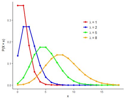
For a given number of events x, the function takes a value of P(X = x) (coordinates of points in the plot), while its shape depends only on the rate parameter, λ. You can easily find out how the probabilities change for different chances of success and the same number of events. Compare P(λ = 2; x = 3) = 0.224 and P(λ = 8; x = 3) = 0.029. The first event is 7.7 times more likely to happen!

On the other hand, when you use the Poisson calculator to find out cumulative probability, you're looking at a certain area below the function. For example, the cumulative probability P(λ = 5; x < 4) = 0.265 is the area on the left from the point P(λ = 5; x ≤ 4) = 0.176, and below the green line. These values can also be found in the Poisson distribution table.

Note that for the lowest values of λ, the Poisson distribution is strongly asymmetric and right-skewed, with highest probabilities assigned to the very first occurrences of an event. When λ increases, the probability distribution gets more evenly dispersed and similar to the well-known bell curve, as implied by the central limit theorem.

You can play around with the Poisson calculator to find how low the probability values become when we consider a large number of events.

Poisson's original formulation of his probability distribution was often called the law of small numbers, as it applies to an event that happens rarely, but has many opportunities to happen. In other words, the chance of success is small, but the number of trials is large.

Interestingly, the Poisson distribution is an extreme case of the binomial distribution, as can be shown by asymptotic properties of the latter.

Poisson himself thought of this statistical tool when he tried to figure out the number of wrongfully convicted by the French judiciary system. The Poisson distribution has since then found various applications.

It was developed to approximate chances of winning random games. Statistician Wladyslaw Bartkiewicz, who made the Poisson distribution formula functional in the late 19th century, famously fitted this model to the data of the number of Prussian cavalrymen accidentally killed by being kicked by a horse. (Apparently, one of the Prussian virtues included reliable data collection).

It was shown for the first time that such uncommon events could be successfully predicted if we estimate just one parameter, λ.

During the Second World War, the Poisson probability definition was effectively implemented in operations research. Military engineers employed it for measuring the accuracy of airstrikes, queuing theory, and network traffic models.

Today the Poisson distribution is used everywhere, from chemistry to economics. You may find it in sophisticated financial models used, e.g. to explore the impact of rare events on efficient portfolio management, or perform stress testing in financial institutions. In particular, it is well-suited to study high impact - low probability events (HILPE) that typically mark the initial phase of financial crises.

Poisson distribution is an example of a discrete distribution, which means that the Poisson distribution table works for only non-negative integer arguments. Unlike continuous distributions (e.g., normal distribution), that may generally take a value of any real number, it can assume only a countably infinite number of values.

What's more, the Poisson distribution calculator shouldn't be used when:

• events are not independent (probabilities of subsequent events change over time);
• there is no chance of an event occurrence (probability function is undefined for zero events).

In the first case, the Poisson probability definition does not correctly work when events are serially correlated. Specifically, you can come across many examples of positive autocorrelation in the data: a volcano eruption that makes other volcanoes more likely to erupt, or an epidemic disease displaying high dynamics.

Additionally, the Poisson distribution must be augmented when we deal with events for which the value of zero cannot occur (e.g., once a patient is hospitalized, they never leave a clinic after zero days). This problem may be alleviated using the so-called trimmed distributions, such as the zero-truncated Poisson distribution, which use only a set of positive integers.