This normal distribution calculator (also a bell curve calculator) calculates the area under a bell curve and establishes the probability of a value being higher or lower than any arbitrary value X. You can also use this probability distribution calculator to find the probability that your variable is in any arbitrary range, X to X₂, just by using the normal distribution mean and standard deviation values. This article explains some basic terms regarding the standard normal distribution, gives you the formula for normal cumulative distribution function (normal CDF), the formula for normal distribution, and provides examples of the normal distribution probability.
📊 Your Real-World Statistics Resource Hub
Discover our full that includes expert articles and reports — all in one place!
Popular reads:
Normal distribution definition
The normal distribution (also known as the Gaussian) is a continuous probability distribution. Most data is close to a central value, with no bias to left or right. Many observations in nature, such as the height of people or blood pressure, follow this distribution.
In a normal distribution, the mean value is also the median (the "middle" number of a sorted list of data) and the mode (the value with the highest frequency of occurrence). As this distribution is symmetric about the center, 50% of values are lower than the mean, and 50% of values are higher than the mean.
Another parameter characterizing the normal distribution is the standard deviation. It describes how widespread the numbers are. Generally, 68% of values should be within 1 standard deviation from the mean, 95% within 2 standard deviations, and 99.7% within 3 standard deviations. This is the empirical rule.
The number of standard deviations from the mean is called the z-score. It may be the case that you know the variance but not the standard deviation of your distribution. However, it's easy to work out the latter by simply taking the square root of the variance.

You can say that an increase in the mean value shifts the entire bell curve to the right. Changes in standard deviation tightens or spreads out the distribution around the mean. In strongly dispersed distributions, there's a higher likelihood for a random data point to fall far from the mean. The shape of the bell curve is determined only by those two parameters.
What is the standard normal distribution?
You can standardize any normal distribution, which is done by a process known as the standard score. This is when you subtract the population mean from the data score and divide this difference by the population's standard deviation. A standard normal distribution has the following properties:
- Mean value is equal to 0;
- Standard deviation is equal to 1;
- Total area under the curve is equal to 1; and
- Every value of variable x is converted into the corresponding z-score.
You can check this tool by using the standard normal distribution calculator as well. If you input the mean, μ, as 0 and standard deviation, σ, as 1, the z-score will be equal to X.
The total area under the standard normal distribution curve is equal to 1. That means that it corresponds to probability. You can calculate the probability that your value is lower than any arbitrary X (denoted as P(x < X)) as the area under the graph to the left of the z-score of X.
Let's take another look at the graph above and consider the distribution values within one standard deviation. You can see that the remaining probability (0.32) consists of two regions. The right-hand tail and the left-hand tail of the normal distribution are symmetrical, each with an area of 0.16. This mathematical beauty is precisely why data scientists love the Gaussian distribution!
The normal CDF formula
Calculating the area under the graph is not an easy task. You can either use the normal distribution table or try integrating the normal cumulative distribution function (normal CDF):
For example, suppose you want to find the probability of a variable being lower than . In that case, you should integrate this function from minus infinity to . Similarly, if you want to find the probability of the variable being higher than , you should integrate this function from to infinity. Make sure to check out the p-value calculator for more information on this topic.
You can also use this calculator as a normal CDF calculator!
Note, however, that the cumulative distribution function of the normal distribution should not be confused with its density function (the bell curve), which simply assigns the probability value to all of the arguments:
By definition, the density function is the first derivative, i.e., the rate of change of the normal CDF.
Formula for normal distribution: an example
The formula for normal distribution is presented in the equation below:
where,
- – the population mean; and
- – standard deviation.
Let us calculate the probability density function by taking as the raw score, , and . With these data in hands we can compute:
How to use the normal distribution calculator: an example
-
Decide on the mean of your normal distribution. For example, we can try to analyze the distribution of height in the United States. The average height of an adult man is 175.7 cm.
-
Choose the standard deviation for your dataset. Let's say it is equal to 10 cm.
-
Let's say you want to use this bell curve calculator to determine an adult's probability of being taller than 185 cm. Then, your will be equal to 185 cm.
-
Our normal distribution calculator will display two values: the probability of a person being taller than 185 cm () and shorter than 185 cm (). In this case, the former is equal to 17.62% and the latter to 82.38%.
-
You can also open the "Range probability" section of the calculator to calculate the probability of a variable being in a particular range (from X to X₂). For example, the likelihood of the height of an adult American man being between 185 and 190 cm is equal to 9.98%.
The amazing properties of the bell curve probability distribution
The normal distribution describes many natural phenomena: processes that happen continuously and on a large scale. According to the law of large numbers, the average value of a sufficiently large sample size, when drawn from some distribution, will be close to the mean of its underlying distribution. The more measurements you take, the closer you get to the mean's actual value for the population.
However, keep in mind that one of the most robust statistical tendencies is the regression toward the mean. Coined by a famous British scientist , this term reminds us that things tend to even out over time. Taller parents tend to have, on average, children with height closer to the mean. After a period of high GDP (gross domestic product) growth, a country tends to experience a couple of years of more moderate total output.
It may frequently be the case that natural variation, in repeated data, looks a lot like a real change. However, it's just a statistical fact that relatively high (or low) observations are often followed by ones with values closer to the average. Regression to the mean is often the source of anecdotal evidence that we cannot confirm on statistical grounds.
The normal distribution is known for its mathematical probabilities. Various probabilities, both discrete and continuous, tend to converge toward normal distribution. This is called the central limit theorem, and it's clearly one of the most important theorems in statistics. Thanks to it, you can use the normal distribution mean and standard deviation calculator to simulate the distribution of even the most massive datasets.
More about the central limit theorem
As your sample size gets larger and larger, the mean value approaches normality, regardless of the population distribution's initial shape. For example, with a sufficiently large number of observations, the normal distribution may be used to approximate the Poisson distribution or the binomial probability distribution. Consequently, we often consider the normal distribution as the limiting distribution of a sequence of random variables.
That's why best practice says that many statistical tests and procedures need a sample of more than 30 data points to ensure that a normal distribution is achieved. In statistical language, such properties are often called asymptotic.
If you're not sure what your data's underlying distribution is, but you can obtain a large number of observations, you can be pretty sure that they follow the normal distribution. It is true even for the random walk phenomena, that is, processes that evolve with no discernible pattern or trend.
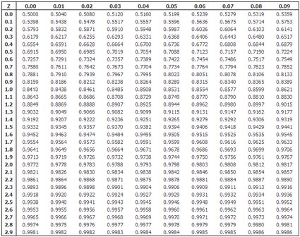
Normal distribution table and multivariate normal
A standard normal distribution table, like the one below, is a great place to check the referential values when building confidence intervals. You can use our normal distribution probability calculator to confirm that the value you used to construct the confidence intervals is correct. For example, if X = 1.96, then X is the 97.5 percentile point of the standard normal distribution. (Set mean = 0, standard deviation = 1, and X = 1.96. See that 97.5% of values are below the X.)
What's more, provided that the observation you use is random and independent, the population mean and variance values you estimate from the sample are also independent. The univariate Gaussian distribution (calculated for a single variable) may also be generalized for a set of variables. A specific "sum" called the shows the joint distribution of a particular number of variables. You may use it to model higher dimensional data, such as a comprehensive assessment of patients.
Normal distribution and statistical testing
Statisticians base many types of statistical tests on the assumption that the observations used in the testing procedure follow the Gaussian distribution. It is valid for nearly all inferential statistics when you use the sample's information to make generalizations about the entire population.
For example, you may formally check whether the estimated value of a parameter is statistically different than zero or if a mean value in one population is equal to the other. Most of the simple tests that help you answer such questions (the so-called parametric tests) rely on the assumption of normality. You cannot use it when an empirical distribution has different properties than a normal one.
You should test this assumption before applying these tests. There are a couple of popular normality tests to determine whether your data distribution is normal. The Shapiro-Wilk test bases its analysis on the variance of the sample. In contrast, the Jarque-Bera test bases it on skewness and the excess kurtosis of the empirical distribution. Both tests allow you for accurate interpretation and maintain the explanatory power of statistical models.
Testing for normality also helps you check if you can expect excess rates of return on financial assets, such as stocks, or how well your portfolio performs against the market. We may use the mean of the empirical distribution to approximate the effectiveness of your investment. On the other hand, you can use the variance to assess the risk that characterizes a portfolio.
One of the most commonly used normality assumptions regards linear (or even non-linear) regression models. Typically, we assume that the least squares estimator's residuals follow a normal distribution with a mean value of zero and fixed (time-invariant) standard deviation (you can think of these residuals as a distance from a regression line to actual data points). You may assess the goodness of fit of the least square model using the chi-square test. However, if the error distribution is non-normal, it may mean that your estimates are biased or ineffective.
Another important example in this area is ANOVA (analysis of variance), used to check whether the mean values of two samples are equal. The ANOVA may also be successfully performed in the canonical form when the distribution of model residuals is normal.
Going beyond the bell curve
There are several ways in which the distribution of your data may deviate from the bell curve distribution, but the two most important of them are:
- Fat tails — extreme values may occur with higher probabilities (e.g., there's a relatively high chance of getting abnormal results);
- Skewness — distribution is asymmetric. The mean and median values of the distribution are different (e.g., dispersion of wages in the labor market).
Non-normal distributions are common in finance, but you can expect the same kinds of problems to appear in psychology or social studies. One of many examples of such distributions is the geometric distribution, suitable for modeling a number of independent events, e.g., the outcome of rolling dice.
FAQs
What is the normal distribution in statistics?
The normal distribution (or Gaussian distribution) is a bell-shaped probability distribution for independent random variables. It is crucial to statistics because it accurately describes the distribution of values for many natural phenomena. The distribution curve is symmetrical around its mean, with most observations clustered around a central peak and probabilities decreasing for values farther from the mean in either direction.
Can a normal distribution have a large standard deviation?
Yes, a normal distribution can have large standard deviation compared to the mean. For example, a normal distribution may have a mean of 6 but a standard deviation of 20. In general, the wider the normal distribution relative to the mean, the larger its standard deviation.
How do I know if data is normally distributed?
To determine if a dataset is normally distributed:
- Draw a graph of the data distribution.
- Check that the curve has the shape of a symmetrical bell centered around the mean.
- Check the empirical rule: 68% of values must fall within 1 standard deviation from the mean, 95% within 2 standard deviations, and 99.7% within 3 standard deviations.
Which are the two main parameters of the normal distribution?
The two main parameters of the normal distribution are: mean (μ) and standard deviation (σ). μ determines the location of the peak of the normal distribution on the numerical axis. σ is a scale parameter that causes the normal distribution to spread out more at larger values of σ.
What percentage of trees will have a circumference greater than 210 cm?
2.5%, assuming that for an oak tree, the normal distribution of the circumference has μ = 150 cm and σ = 30 cm.
- Draw the normal distribution with the peak at μ = 150 cm and σ = 30 cm.
- Note that the 210 cm circumference is 2σ = 60 cm above the mean.
- Use the empirical rule that 95% of the data lies within ±2σ.
- Divide by 2 to take the trees with a circumference over +2σ.