Hohmann Transfer Calculator

The Hohmann transfer calculator can help you find the transfer trajectory requiring the minimum amount of propellant (fuel and oxidizer) to go from one circular orbit to another. Our calculator can quickly find characteristics of the Hohmann transfer, including delta-v. Do you have a rocket engine with you? Our calculator can also provide you required mass of propellant for a Hohmann transfer.

Are you hearing about Hohmann's transfer for the first time? Are the words "Hohmann transfer delta-v calculation" and "Hohmann transfer orbit" confusing, or are you curious and want to understand what all the fuss is about a Hohmann transfer? If yes, the article below is a perfect place to understand all the concepts with Hohmann transfer examples. Please continue to read on!

Before you start reading our article, we would like to give you a chance to ponder about the Hohmann transfer and its application. Let us say you are the commander of a spaceship that needs to go from Earth to Mars. Your spacecraft uses chemical propulsion, and you want to know how much propellant (including both fuel and oxidizer) is needed for the travel.

What are the assumptions you can make on the nature of Earth's and Mars's orbit such that you can make use of Hohmann transfer? Okay! Do not worry if you do not know the answer yet. We assure you that you will know the answer by the end of the article (psst! the answer is given at the end of this article).

To use our calculator, you need very few details:

1. First, you should know your primary body characteristics: Mass and radius.
   • Note: You can use our unit switcher to change the mass unit to "Weights of Earth" if your primary body is Earth or to "Weights of Sun" if it is Sun (by doing this, you are measuring your mass in terms of multiples of the mass of the Earth or Sun).
2. Next is your initial and final orbit's altitude from the surface of the primary body.
3. With these pieces of information, our Hohmann transfer calculator will provide you details about the Hohmann transfer orbit's (or transfer ellipse) properties, delta-v ($ΔV$).
4. After delta-v calculation, if you have your rocket engine's $I_{\mathrm{sp}}$ and initial mass, our calculator also embeds the rocket equation that provides you with the amount of propellant needed for the transfer.
5. At the bottom of some sections, we have a further properties option. You can use them to get more details, such as specific angular momentum and geometrical properties of the initial, destination, and transfer orbit.

To directly see the example of Hohmann transfer, please go to traveling from Earth to Mars by using Hohmann transfer calculator section of this article.

Astrodynamics

Astrodynamics is the field of physics that deals with the study of the motion of artificial objects under the influence of the gravitational field of one or more natural bodies. Knowledge of astrodynamics is used in interplanetary trajectory design (e.g., Earth to Mars), constellation design of satellites for navigation, communication, Earth observation, futuristic space tourism, etc.

Trajectory of an object

The path traversed by an object in space is called its trajectory. For example, the Moon crosses a circular trajectory around the Earth. The object can traverse two different types of trajectories. In astrodynamics, the motion of an object under the influence of a single primary body is called a two-body problem and is characterized by conic sections. In the figure below, you can see that by cutting the right circular cone at different angles, we get two different trajectories (Kepler orbits).

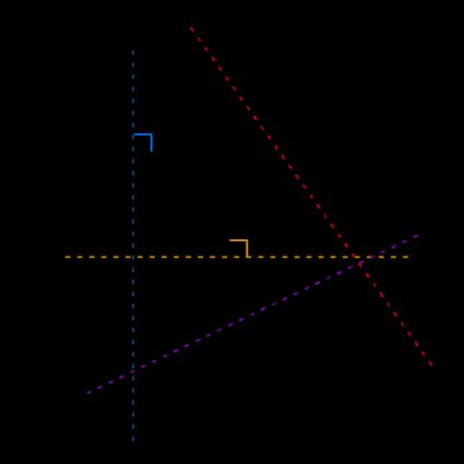
Two trajectories are described below:

• Open trajectories – When the plane passing through the cone base cuts the cone, either perpendicularly (line $H^1-H$ in the above figure) or at an inclined angle to the horizontal axis (line $P^1-P$), we end up having either a hyperbola or a parabola, respectively. The figure shows it clearly.
• Closed trajectories – When the plane cuts the cone, either perpendicular (line $C^1-C$) or at an inclined angle(line $E^1-E$) to the vertical axis, we end up having either a circle or an ellipse, respectively. Velocity at each point on a circle is always tangential, whereas for ellipse only at the perigee (p) and apogee (a) are extreme points on the ellipse, the velocity is tangential. These properties are used by Hohmann transfer to calculate the best fuel-efficient transfer. Please check out our ellipse calculator to learn more about ellipse.

Specific angular momentum

Specific angular momentum is defined as the angular momentum divided by its mass. Each orbit is characterized by specific angular momentum that remains constant. It is given by the cross product between position vector $\vec r$ and velocity vector $\vec v$, i.e., $\vec h=\vec r \times \vec v$. Below, we have equations to compute the magnitude of $\vec h$ for circular and elliptical orbits:

• Elliptical orbit: The magnitude of specific angular momentum equation is given as:

where:

• $\mu$ – Gravitational parameter defined as the product between the primary object's mass $M$ and gravitational constant $G$, i.e., $\mu=GM$. For Earth, $\mu$ is $398600.418\ \text{km}^3/\text s^2$; and

• $r_\mathrm{a}$ and $r_\mathrm{p}$ are the apogee ($\mathrm{a}$) and perigee ($\mathrm{p}$) radii of an ellipse respectively.

• Circular orbit: Circular orbit case is a special case of elliptical orbit when the $r_a$ and $r_p$ are equal. Thus, the equation of $h$ becomes $h=\sqrt{\mu r}$. If the orbital velocity is known for a circular orbit, you can use the fundamental definition of specific angular momentum $h$, given by $h= rv$.

You can calculate the orbital velocity using simple formulas from rotational motions or using our orbital velocity calculator!

Specific impulse

If you want to compare the performances of two rocket engines, you will first look at their specific impulse. Specific impulse ($I_{sp}$) is the parameter that tells us how much thrust a rocket is producing per unit rate of propellant weight. It is given by:

where:

• $T$ — Thrust produced by a rocket in $\mathrm{N}$;
• $\dot m_\mathrm{p}$ is the rate of propellant consumption in $\text{kg/s}$; and
• $g_\mathrm{o}$ is the acceleration due to gravity at sea level on Earth (also called as standard acceleration due to gravity) in $\text{m/s}^2$.

The unit of specific impulse is the second ($\mathrm{s}$).

Transfers are essential aspects of astrodynamics used to move an object from one point to another in space. Specifically, this article focuses on transfers between two closed orbits (also known as periodic orbits) called orbital transfers. In the following paragraphs, let us understand different orbital transfers present in the literature.

The orbital transfer is the transfer of spacecraft from one to another orbit. For example, moving a spaceship from a circular orbit to another circular orbit. Based on the thrusting strategies used while transferring, orbital transfers can be divided into two types, they are:

Impulse transfer

Impulse transfers are the transfers whose thrusting time $t$ is very small compared to the time of flight $\text{ToF}$ (also known as the total transfer time). All of the transfers before electric propulsion technology were impulse transfers that were accomplished using chemical rocket propulsion. This transfer requires a tremendous amount of fuel, but you will reach the destination orbit in a reasonable time (as compared to a "low thrust transfer"). Hohmann transfer is one of the impulse transfer strategies. We will see this in some detail later in the article.

Low thrust transfer

Low thrust transfers are the transfers whose thrusting time $t$ is not too small compared to the time of flight $\text{ToF}$. Currently, there is a shift in the space industry to use electric propulsion technologies as it avoids carrying the enormous amount of propellents onboard the spacecraft. This advantage comes at a price. The price is that the electric propulsion imparts only a small amount of momentum onto the spacecraft; as a result, you will require more time to reach your destination.

Before going into details of the Hohmann transfer, let us take a detour and understand the famous equation in rocket science.

You have a rocket engine that uses chemical propulsion (once the rocket is chosen, its performance parameter $I_{\mathrm{sp}}$ is fixed). To understand how far the rocket can go using the available propellant, $m_\mathrm{p}$ is provided by the Tsiolkovsy rocket equation.

The delta V is given by:

where:

• $ΔV$ – Maximum velocity that can be imparted to the spacecraft in $\text{m/s}$. This critical quantity indicates how much change in velocity a rocket engine can impart and has commonly called "delta-v" pronounced as "delta-vee" in the space industry;
• $I_{\mathrm{sp}}$ – Specific impulse in $\mathrm{s}$;
• $g_\mathrm{0}$ – Standard acceleration due to gravity at sea level on the earth in $\mathrm{m/s^2}$;
• $m_0$ – Initial mass of the rocket in $\text{kg}$; and
• $m_\mathrm{f}$ – Final mass in $\text{kg}$ at burn-out time $t_{\mathrm{b}}$ after consuming all the propellants $m_\mathrm{p}$, i.e., $m_\mathrm{f}=m_0-m_\mathrm{p}$.

This equation is valid only for impulse transfers; the burnout time $t_\mathrm{b}$ is much shorter than the time of flight ($\text{ToF}$).

In situations, where required $ΔV$ is known already for a given $I_{\mathrm{sp}}$ and initial mass $m_0$ of the rocket, the propellant mass $m_\mathrm{p}$ can be found by using:

We will make use of this equation later in the article. Now that we have learned about the rocket equation and $ΔV$, it is the right time for us to go back to impulse transfer and look at Hohmann orbit transfer.

A Hohmann transfer is a type of impulse transfer that requires minimum fuel to move an object from one circular orbit to another. Essentially, we have two circular orbits; one is our initial orbit, and another is the destination. These two orbits will be connected by an orbit called a transfer orbit or Hohmann transfer orbit. In a Hohmann transfer, the transfer orbit is an ellipse.

A Hohmann transfer includes two $ΔV$ (thrustings) as shown in the figure below. As you can expect, there are two scenarios involving a Hohmann transfer. One is where you move your object from lower to a higher altitude orbit (subfigure a), and another is from higher to lower altitude orbit (subfigure b).

In both cases, the total $ΔV$ magnitude is the same. We can notice from the figure the only difference is the direction of application of $ΔV$. In the following paragraphs, we consider only subfigure a scenario for further analysis.

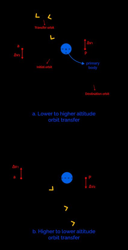
First, $ΔV_1$ is applied at a point $\mathrm{p}$ on the initial orbit, forming the perigee of the transfer ellipse. Let $v_{1_\mathrm{p}}$ be the velocity at a point $\mathrm{p}$ on the initial orbit. To transfer the object to Hohmann transfer orbit at point $\mathrm{p}$, where the velocity is $v_{\mathrm{t_p}}$ on the transfer orbit, we need an extra velocity increment given by $ΔV$. The following equations are used to find $ΔV$ at point $\mathrm{p}$.

First, velocity $v_{1_\mathrm{p}}$ on the initial orbit is given by:

where:

• $h_1$ – Specific angular momentum of the initial orbit in $\text m^2/\text s$; and
• $r_{1_\mathrm{p}}$ – Radius of initial orbit at $\mathrm{p}$ in $\text m$; since its a circle $r_{1_\mathrm{p}}$ is the same at every point.

Now, the transfer orbit's velocity $v_{\mathrm{t_p}}$ at point $\mathrm{p}$ is given by:

where:

• $h_\mathrm{t}$ — Specific angular angular momentum of transfer orbit in $\text m^2/\text s$;
• $r_{\mathrm{t_a}}$ and $r_{\mathrm{t_p}}$ — Apogee and perigee radius of an ellipse in $\text m$, respectively; and
• $\mu$ — Gravitational parameter in $\text{km}^3/\text s^2$.

Therefore the magnitude of $ΔV_1$ is given as:

After the first $ΔV_1$, the object travels through the transfer orbit and reaches point $\mathrm{a}$, which is the apogee of the transfer orbit. Once we are at a point $\mathrm{a}$ on the destination orbit, the second $ΔV$ is applied, which forms the apogee of the transfer ellipse.

Similarly, in this case, to move the object from transfer ellipse to destination orbit, we increment the velocity of the transfer ellipse $v_{\mathrm{t_a}}$ at $\mathrm{a}$ to match the velocity of the destination orbit $v_{2_\mathrm{a}}$ using second $ΔV_2$. The following equations are used to find $Δ V_2$ at point $\mathrm{a}$.

First, velocity $v_{\mathrm{t_a}}$ on the transfer orbit at point $\mathrm{a}$ can be found just by replacing the $r_{\mathrm{t_p}}$ term of the denominator of equation 7 by $r_{\mathrm{t_a}}$ and it is given by:

Finally, destination orbit's velocity $v_{2_\mathrm{a}}$ at a point $\mathrm{a}$ by using:

where:

• $h_2$ — Specific angular momentum of initial orbit in $\text m^2/\text s$; and
• $r_{2_\mathrm{a}}$ ‚ Radius of destination orbit at a in $\text m$; since its a circle $r_{2_\mathrm{a}}$ is the same at every point.

Therefore, the $ΔV_2$ is given as:

Now that we have two $Δ V$'s at $\mathrm{p}$ and $\mathrm{a}$, our final total $ΔV_{\text{total}}$ is given as:

The figure shows the Hohmann transfer to move from a lower circular orbit to a higher one (commonly called orbit raising in space industry jargon).

In essence, a Hohmann transfer provides the $ΔV$ required at each point, i.e., $\mathrm{p}$ and $\mathrm{a}$, which happens to be the perigee and apogee of the transfer orbit to move an object from one orbit to another.

The analysis is very much similar for transfer from higher to lower altitude orbit. The result will show changes only in the sign of obtained $ΔV$ indicating the change in the direction of application.

Amount of propellant required

Once we have the $ΔV$ for our transfer, we can make use of the rocket equation that we saw in our rocket equation and "delta-v" section to find the amount of propellant required:

We want you to be an efficient and smart spaceship commander for this Hohmann transfer example. Thus, we provide you with the following checklist to help you see if you can use our Hohmann transfer to Mars calculator:

• Initial and final orbit must be circular: Are your orbits circular?

  Earth and Mars orbit's eccentricity values are 0.0167 and 0.0934, respectively. Therefore, they can be assumed to be circular orbits.

• Initial and final orbit must be in the same plane (or co-planar): Are your orbits co-planar?

  Earth and Mars orbit's inclinations are 0° and 1° 51' 09'', respectively, with respect to the ecliptic plane. Since they are close to 0°, we can approximate their orbits to be co-planar.

• The rocket engine works on the impulsive principle: Is your rocket engine a chemical propulsion or impulsive type?

  The spaceship is making use of chemical propulsion; as a result, we can consider it impulsive type propulsion.

If all of the above checklists are satisfied, you can use our Hohmann transfer calculator.

Note: Since you are moving from Earth to Mars orbit, the scenario is the lower altitude to higher altitude orbit Hohmann transfer. It corresponds to the subfigure b in the Hohmann transfer and delta-v calculation section.

The following data needs to be inserted:

• First, you have to choose the primary body. For Earth to Mars travel, the primary body is the Sun. If you are dealing with satellites revolving around Earth, the primary body is Earth. According to that, the values of the mass and radius of the primary body are inserted into the fields:

  • Mass of the Sun: $1.989\times10^{30}\ \text{kg}$
  • The radius of the Sun: $696,340\ \text{km}$

• Next, in the initial orbit section, enter the object's altitude from the surface of the primary body. Our initial orbit is the Earth's orbit:

  • Altitude: $146,403,660\ \text{km}$

• With altitude, our calculator will provide you with the specific angular momentum and velocity at point $\mathrm{p}$ (you can check them in the further properties sections of our Hohmann transfer calculator). Now we are dealing with Earth and Mars, "altitude" may sound strange, but it can be easily computed once you know the distance of either planet from the center of the Sun.

• Furthermore, we have a destination orbit section. Enter the altitude of Mars orbit from the surface of the Sun:

  • Altitude: $206,\!003,\!660\ \text{km}$

With the above data, our Hohmann transfer calculator will find the Hohmann transfer orbit properties to Mars and corresponding $ΔV$s, as shown in the table below.

Knowing the $ΔV$, we can find the propellant mass $m_\mathrm{p}$ required, for that impulse $I_{\mathrm{sp}}$ and the initial mass ($m_0$) of your spaceship in the Required mass of the propellant section:

• $I_{\mathrm{sp}} = 400\ \mathrm{s}$
• $m_0 = 200,\!000\ \mathrm{kg}$

The propellant mass you need to carry on your spaceship is $139,105.04\ \mathrm{kg}$.
With these results in mind, you will be able to command your spaceship to Mars!

Awesome! We hope you have enjoyed reading our article and the Hohmann transfer to Mars calculator. Now that you know how to go to Mars, check out our space travel calculator, which will help you understand how far we can go in this vast cosmos!

Ad Astra! 😀