Queueing Theory Calculator

Q: What is queueing theory?

Queueing theory is a mathematical framework created to explain waiting lines. You need some fundamental elements to define a queue: An arrival statistics (how the queues grow); The servicing rate (how the queue shrinks); and The number of servers. In the most common queue, both the intervals between successive arrivals and the servicing times are described by exponential distributions, and there is a single server. The corresponding model is the M/M/1 queue. Read more

Q: What is the condition for a queue to eventually end?

A queue ends if and only if the service rate exceeds the customers' arrival rate. This way, the servers allow the queue of customers to eventually deplete. A good measure of this attitude is the traffic intensity, the ratio between arrival and servicing rate. The lower the rate, the easier the flow of the queue. Read more

Q: What is the average waiting time in an M/M/1 queue with ρ = 0.17 and λ = 0.03

6.83 . To calculate this value, follow these steps: Find the servicing rate μ : μ = λ/ρ = 0.03/0.17 = 0.17647 . Plug the appropriate values in the formula for the time in the system: W = 1/(μ - λ) : W = 1/(μ - λ) = 1/(0.17647 - 0.03) = 6.83 To find the value of the actual waiting time, multiply the result by ρ = λ/μ : Wq = ρ × W = 0.17 × 6.83 = 1.16 This time consider only the time you are standing in line. Read more

Q: What is the most common policy used to service a queue?

As you can imagine, the most common policy to service a queue is the first-in-first-out one. This method is applied in almost every system where humans queue, and for all the right reasons! However, there are exceptions. In priority-based systems, this policy has many shortfalls. Similarly, the policy last-in-first-out appears when, for example, we are leaving a crowded bus. The answer is: it depends! Read more

Created by Davide Borchia

Reviewed by Anna Szczepanek, PhD and Adena Benn

Last updated: Jan 18, 2024

Table of contents:

In the last century, mathematicians developed a framework that describes the dynamics of a waiting line: learn the fundamentals of queueing theory with our queueing theory calculator.

Since humans started getting along in that thing we call society, they also started waiting. Waiting for their turn to talk, eat, pay taxes, you name it. With the growth of the population and the increasing complexity of our daily lives, we started waiting even more.

It's not surprising that someone developed an interest in analyzing and modeling the behavior of queues. Understanding how long it will take to clear a line of customers or how many checkouts to keep open during a busy afternoon is a real help in smoothing many time-consuming processes.

Now you can imagine why queueing theory is important: keep reading to learn more. In this article, you will discover:

The fundamentals of queueing theory: what is queueing theory?
The principal elements of a queue and the Kendall notation;
The cornerstone of queues: the $\textbf{\text{M}/\text{M}/1}$ queue;
Adding servers: the $\textbf{\text{M}/\text{M}/s}$ queue;
How to use our queueing theory calculator, with examples; and
Applications of the queueing theory.

This article is nothing but a dent in the surface of the intriguing framework of queueing theory. If interested, we invite you to expand from here! What are you waiting for? Pun intended. 😉

What is queueing theory?

You don't have to spend weeks on a thick book to understand what queueing theory is — though its mathematical description may get pretty long: we are talking of the same process of entering a waiting line — and waiting — to get access to a service. You do this every time you get groceries or go to the bank.

The queueing theory was developed by Agner Krarup Erlang in the early XX century while he was waiting in line at a slow local post office. No, sorry, while he was working on the analysis of telephone networks. The theory successfully developed in the following years, thanks to the pervasive nature of queues and the helpfulness of the results of the queueing models.

So, what exactly is the queueing theory? The queueing theory analyzes the behavior of a waiting line to make predictions about its future evolution. Some examples of what we can calculate with a queueing model are:

The waiting and service time;
The total number of customers in the queue;
The utilization of the server.

And much more.

Queueing theory has deep roots in statistics and probability. The arrival and servicing of customers are, fundamentally, stochastic processes. However, when analyzing such processes over long times or far in the future, their implicit randomness somehow vanes: we talk then of the steady state of the process. A detailed description of the foundations of queueing theory requires a solid background in the mentioned field of maths: we will try to keep it low and focus on the calculations for the queueing theory models!

When do we use queueing theory?

Queueing theory has many applications, and not only where humans wait! The management of the take-offs and landings at a busy airport, the execution of programs on your computer, and the behavior of an automatized factory all benefit from a careful analysis of queues.

From calculating traffic density to graphing theory, queues are everywhere, from theoretical mathematics to our daily lives!

Speaking of...

What is a queue?

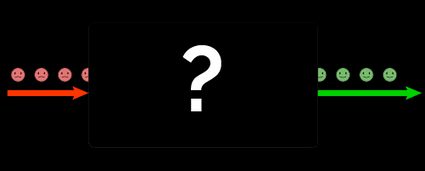
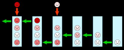
In the mathematical sense, a queue is a complex object modeled by a black box. In this black box, we identify two flows: one inbound and one outbound. What happens inside the box is unknown, but the outbound customers are happier than the inbound ones.

A queue black box — What happens inside the box?

If we peek inside the box, we see a certain number of servers that process the request of the customers. Some are free — waiting to receive a customer, and some are currently busy. One way or the other, the queue moves on.

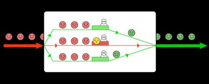
Inside the box there are three mustachoed servers

What matters to the modelization of a queue is usually the customers' waiting time. Say you want to optimize it or to find pitfalls that uselessly prolong it. Other goals are to optimize the "utilization" of servers or decrease the queue length.

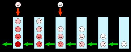
Describing a queue in the mathematical sense requires understanding some basic concepts. Firstly, a queue is represented by states, each telling us the number of people in the queue, either waiting or being serviced.

A birth and death process — We can represent a queue with a birth and death process.

With certain probability — a quick reminder that queues are rooted in the framework of stochastical processes — the customers arrive and receive the required service. This moves the queue: arrivals increase the state, and services reduce it to reach the state $0$ .

🙋 If you've already met Markov chains, then yes, the representation of a queue lives in this framework. We consider queues to be Markovian processes in a stable state.

States are related to probabilities, but the queue theory describes the time spent in a given state more than defining this quantity. An alternative explanation is the chance of having a specified number of customers in the queue: time and "occupation" are, surprisingly, equivalent!

Queueing discipline: who's going first?

The order in which customers receive service in a queue is the queueing discipline. The most common discipline is the first in, first out discipline (FIFO), where the customer priority depends on the time spent in the queue.

A reasonable policy — The first-in-first-out policy is the one we are used to: look at how natural it feels.

Other disciplines are:

Last in first out (LIFO), where items entered last are the first ones to be serviced. Think of a pile of pancakes or things stuffed in a backpack. This discipline is rarely used when humans are involved: we let you guess why!
Priority discipline happens when the servicing order depends on some defining factors. In the ER, the man with an alien poking out of his chest will pass before the one who hit his pinky on a corner: they may even use our injury severity score calculator to assess a patient's priority.
Round robin servicing, where the customer receives service for a given time and can re-enter the queue; and
Service in random order (SIRO), that no one likes.

lifo queue — That's the evilest thing we can imagine! A queue where the last to enter is the first to exit, according to the LIFO policy..

Most models, and all the ones we will analyze here, use the FIFO discipline — it's the most reasonable!

Priority servicing — The redder the smiley, the higher the priority. This policy considers the urgency required by a customer.

Meet the servicing policies in other fields at Omni's fifo calculator and lifo calculator!

The Kendall notation: classifying queues

How do we identify a queue? David George Kendall answered this question by laying down a straightforward notation that helps to choose the right set of equations for each situation quickly. The basic Kendall notation consists of three symbols in the form:

a/b/c

Where:

$a$ is the probability distribution for the intervals between customer arrivals;
$b$ is the probability distribution of the servicing time; and
$c$ is the number of servers.

$a$ and $b$ can assume various values (letters), the most important being:

$\text{M}$ , standing for Exponential distribution;
$\text{E}$ , standing for Erlang distribution;
$\text{G}$ for any general probability distribution of which you know mean and variance.

You can expand the Kendall notation to include other parameters. The notation $a/b/c/d/e/f$ includes:

$d$ the maximum number of customers accepted in the queue (think of the capacity of an office);
$e$ the size of the customer population; and
$f$ the queueing discipline.

The most commonly analyzed queue is the $\text{M}/\text{M}/1$ queue (exponential distribution for the intervals between arrivals and servicing times by a single server). We will describe it in detail. Other commonly studied queues are the $\text{M}/\text{M}/\text{s}$ and $\text{M}/\text{M}/\text{s}/\text{N}$ .

The M/M/1 queue: your first example of a queueing theory model

We can analyze some models now that you know what queueing theory is. Here we will deal with the simplest queueing model. Take a single queue with a single server, and assume that:

The time intervals between successive customers' arrivals follow an exponential distribution; and
The servicing times follow an exponential distribution.

Poisson and exponential probability distributions are closely related concepts. Considering a Poisson process (a stochastic process describing random occurrences of an event): the number of events in a given time follows the Poisson distribution. The interval between those events, on the other hand, follows the exponential distribution.

In the context of an $\text{M}/\text{M}/1$ queue, this means that the time of arrival of each customer is independent of the other (no rush hours or downtimes), and the time interval between arrivals, $t_{\mathrm{a}}$ follows this distribution:

f(t) = \lambda\mathrm{e}^{-\lambda t}

The servicer takes a specific time for each request, $t_{\mathrm{s}}$ that doesn't depend on previous or future events (e.g., the service of a late customer won't go faster because dinner time approaches!). The distribution takes this form:

g(t) = \mu\mathrm{e}^{-\mu t}

Arrival and service allow us to move the queue between states, balancing each other or prevailing; they make our system dance.

🙋 Queues are inherently memoryless: the past and future events (in our case, the arrival of a customer and the completion of a service) follow two types of processes defined by this lack of influence of previous states: the Markov chains and the exponential distributions.

If we move in the steady-state, we can define the two fundamental quantities we've just met in the formulas for the distributions:

The arrival rate $\lambda$ , which describes the number of customers entering the queue per unit of time; and
The service rate $\mu$ , the number of serviced customers per unit of time.

$\lambda$ and $\mu$ describe how the queue moves between states, interplaying with the fraction of time spent in the state $n$ , $p_{n}$ (with $n$ the number of customers in the queue at that time). We follow these rules:

\mu p_1=\lambda p_0

$\mu p_1$ represents a queue with one customer receiving service, leaving it empty. It corresponds to the opposite process, a customer entering an empty queue ( $\lambda p_0$ ).

For further states, we find:

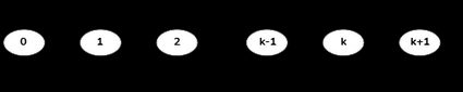
\begin{align*} \lambda p_0+\mu p_2&\!=\!(\lambda\!+\!\mu)p_1\\ \lambda p_{n-1}\!+\!\mu p_{n-1}&\!=\!(\lambda\!+\!\mu)P_{n-1} \end{align*}

How do we find these relationships? By using the previously found equivalence, and an analysis of the queue representation, we can equate the sum of the "arrows" inbound and outbound from a given state. Take a look at the diagram below:

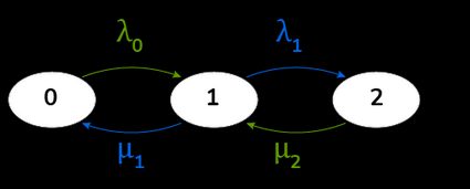
That's how the queue moves. By computing the ratio between the arrival rate and the service rate, we find the traffic intensity $\rho$ :

\rho = \frac{\lambda}{\mu}

🙋 The only condition we need to state for an $\text{M}/\text{M}/1$ queue is that $\lambda<\mu$ , which implies that the queue eventually dies out and doesn't accumulate infinite customers.

Let's analyze the performance measures of the queue. We start with the average number of customers, $L$ .

L=\frac{\rho}{1-\rho}=\frac{\lambda}{\mu-\lambda}

We can now use Little's law to derive the average time spent in the system, $W$ :

\begin{align*} W&= \frac{L}{\lambda}=\frac{\rho}{\lambda(1-\rho)}\\ & =\frac{\lambda}{\lambda(\mu-\lambda)} = \frac{1}{\mu-\lambda} \end{align*}

The time spent in the queue is of equal interest. We denote it as $W_{\text{Q}}$ and calculate it again using Little's law, but this time starting from the number of customers in the queue $L_{\text{Q}} = \rho L$ :

\begin{align*} W_{\text{Q}}&= \frac{L_{\text{Q}}}{\lambda}=\frac{\rho L}{\lambda}=\frac{L}{\mu}\\ & =\frac{\lambda}{\mu(\mu-\lambda)} \end{align*}

The four queue equations we met define the fundamental quantities in every queueing theory model.

What else can be helpful in the analysis of an $\text{M}/\text{M}/1$ ? We can define the probability of no customers in the system, $p_0$ :

p_0 = 1-\rho = 1-\frac{\lambda}{\mu}

We calculate the probability of the presence of $n$ customers in the queue, $p_{n}$ by taking $\rho^n$ times $p_0$ :

p_{\text{n}} = \rho^np_0

What about the values of $p_n$ for any other $n$ ? The formula is straightforward, and it derives from multiple applications of the transition between states from the empty queue:

p_n = (1-\rho)\rho^n

Now that we have analyzed the $\text{M}/\text{M}/1$ queue, we can move to slightly more complex models.

A new checkout opens: the M/M/s queues

We will now analyze an $\text{M}/\text{M}$ queue with several servers bigger than one. We need to introduce a few more quantities here.

$s$ is the number of servers in the system. Each serves independently, following the same exponential distribution and rate of service $\mu$ .

We redefine the server utilization $\rho$ as $\rho = \tfrac{\lambda}{s\mu}$ . You can think of $s\mu$ as the maximum service rate. In fact, an $\text{M}/\text{M}/s$ queue is nothing but an $\text{M}/\text{M}/1$ queue with service rate $s\mu$ .

Let's introduce one last quantity, $\alpha = \tfrac{\lambda}{\mu}$ (which corresponds to the server utilization in the $\text{M}/\text{M}/1$ queue), thus $\rho = \tfrac{\alpha}{s}$ .

However, please pay attention to the behavior of the servicing process. In the $\mathrm{M/M/s}$ queue, we can find situations where some servicers are simply... hanging out, waiting for a customer to arrive. We slightly tweak our definition of $\mu$ in this situation:

\mu_n=\begin{cases} n\mu\ \mathrm{if}\ 1\leq n<s\\ c\mu\ \mathrm{if}\ n\geq s \end{cases}

The steady-state probability of having zero customers in the queue depends, as you can imagine, on the number of servers. We calculate $p_0$ with the formula:

p_0\!=\!\left[\sum_{r=0}^{s-1}\frac{\alpha^r}{r!}\!+\!\frac{\alpha^s}{s!}\left(1\!-\!\frac{\alpha}{s}\right)^{\!-1\!}\right]^{-1}

The number of customers in the queue and in the system, respectively $L$ and $L_{\text{q}}$ , are the results of the $\text{M}/\text{M}/s$ queue equations:

\begin{align*} L &= \alpha\!+\!\frac{\rho\ \!\alpha^s\ \!p_0}{s!\ \!(1-\rho)^2}\\ \\ L_{\text{q}}&= \frac{\rho\ \!\alpha^s\ \!p_0}{s!\ \!(1-\rho)^2} \end{align*}

Let's calculate the waiting times. We do it similarly to the $\text{M}/\text{M}/1$ queue, but we need to modify them slightly.

The waiting time in the system and in the queue are:

\begin{align*} W &= \frac{1}{\mu}\!+\!\frac{\alpha^s\ \!p_0}{s!\ \!s\ \!\mu\ \!(1-\rho)^2}\\ \\ W_{\text{q}} &= \frac{\alpha^s\ \!p_0}{s!\ \!s\ \!\mu\ \!(1-\rho)^2} \end{align*}

We can introduce one last quantity specific for the $\text{M}/\text{M}/s$ queue: the probability of a customer joining the queue and finding no free servers. We call this quantity probability of customer delay, $C(s,\alpha)$ :

C(s,\alpha)=\frac{\alpha^s}{s!}\cdot\left(1-\frac{\alpha}{s}\right)^{-1}\cdot K

$K$ is a parameter we've already met, though slightly different:

K\!=\!\left[\sum_{r=0}^{s-1}\frac{\alpha^r}{s!}\!+\!\frac{\alpha^s}{s!}\left(1\!-\!\frac{\alpha}{s}\right)^{\!-1\!}\right]^{-1}

Eventually, we can define the probability of the queue to be in the state $n$ : we met this quantity before. Since the behavior of this queue depends on the number of customers and servers:

p_n=\begin{cases} \displaystyle{\frac{\lambda^n}{n!\mu^n}}p_0\\[1em] \displaystyle{\frac{\lambda^n}{s^{n-s}s!\mu^n}}p_0 \end{cases}

Now, it's time to meet our queueing theory calculator!

How to use our queueing theory calculator

Our queueing theory calculator allows you to calculate the results of $\text{M}/\text{M}/1$ queues and $\text{M}/\text{M}/s$ queues.

The framework of queueing theory is rather complex: this short article is nothing but an introduction, and our calculator is pretty basic! You can explore it if you just found this exciting branch of mathematics or use it to check the results of your calculations (in particular for queues with multiple servers).

First, choose the queue you are interested in. Input the values you know; we will calculate the rest. Notice that certain operations are hard to invert: $p_0$ for an $\mathrm{M/M/s}$ queue contains a summation and a factorial, and even with all the efforts, we wouldn't be able to use this value as an input. It is greyed out with the other "difficult" values in our queueing theory calculator.

FAQ

What is queueing theory?

Queueing theory is a mathematical framework created to explain waiting lines.
You need some fundamental elements to define a queue:

An arrival statistics (how the queues grow);
The servicing rate (how the queue shrinks); and
The number of servers.

In the most common queue, both the intervals between successive arrivals and the servicing times are described by exponential distributions, and there is a single server. The corresponding model is the M/M/1 queue.

What is the condition for a queue to eventually end?

A queue ends if and only if the service rate exceeds the customers' arrival rate. This way, the servers allow the queue of customers to eventually deplete.

A good measure of this attitude is the traffic intensity, the ratio between arrival and servicing rate. The lower the rate, the easier the flow of the queue.

What is the average waiting time in an M/M/1 queue with ρ = 0.17 and λ = 0.03

6.83. To calculate this value, follow these steps:

Find the servicing rate μ: μ = λ/ρ = 0.03/0.17 = 0.17647.
Plug the appropriate values in the formula for the time in the system: W = 1/(μ - λ):
W = 1/(μ - λ) = 1/(0.17647 - 0.03) = 6.83
To find the value of the actual waiting time, multiply the result by ρ = λ/μ:
Wq = ρ × W = 0.17 × 6.83 = 1.16

This time consider only the time you are standing in line.

What is the most common policy used to service a queue?

As you can imagine, the most common policy to service a queue is the first-in-first-out one. This method is applied in almost every system where humans queue, and for all the right reasons!

However, there are exceptions. In priority-based systems, this policy has many shortfalls. Similarly, the policy last-in-first-out appears when, for example, we are leaving a crowded bus. The answer is: it depends!

Davide Borchia

Type of queue

M/M/1

Arrival rate (λ)

Service rate (μ)

Traffic intensity (ρ)

Average number of customers (L)

Number of customers in the queue (LQ)

Average time spent in the system (W)

Time spent in the queue (WQ)

Probability of no customers in the queue (p0)

The probability of a queue with

customers...

...is pn=

2D distance30 60 90 triangle3 sides triangle area… 657 more

Queueing Theory Calculator

What is queueing theory?

When do we use queueing theory?

What is a queue?

Queueing discipline: who's going first?

The Kendall notation: classifying queues

The M/M/1 queue: your first example of a queueing theory model

A new checkout opens: the M/M/s queues

How to use our queueing theory calculator

FAQ

What is queueing theory?

What is the condition for a queue to eventually end?

What is the average waiting time in an M/M/1 queue with ρ = 0.17 and λ = 0.03

What is the most common policy used to service a queue?

Car heat

Round to the nearest integer

Sinh

Test grade