Parrondo's Paradox Calculator

The Parrondo's paradox calculator will illustrate how two losing games can combine to produce a winning game. This apparently contradictory statement is what Spanish physicist Juan Parrondo discovered while studying the Brownian Ratchet, a thought experiment in the field of physics.

In this calculator, you will find a simulation of Parrondo's paradox as it emerges from a loaded coin-tossing game, which you can experiment with to test this paradox.

We also included a brief mathematical description of how this situation develops using Markov chains and that Parrondo's paradox is, in fact, not so paradoxical.

Keep reading to learn more!

Parrondo's paradox describes the situation where two losing games can be mixed to produce a winning game in the long run. Although this winning strategy needs a particular setup to be feasible, it still has many applications in different fields, such as economics, game theory, and biology.

Let's picture a scenario where you are given two games (game A and game B) that you can play repeatedly. Every time you win in either game, you earn $1. Otherwise, you lose $1.

• Game A: In this game, you will toss an almost fair coin. Your winning odds here are $\text{P}(A) = 0.495$, which is slightly lower than 50/50 and leads to a guaranteed loss in the long run.

• Game B: Before playing, you look at your current capital. If it's a multiple of 3, you play game B₁. If it's not, you play game B₂. In both B₁ and B₂, you will use a loaded coin — however, the odds differ significantly:

  • In game B₁ (when your capital is a multiple of 3) your probability to win is $\text{P}(B_1) = 0.095$.
  • In game B₂ (when your capital is not a multiple of 3) your probability to win is $\text{P}(B_2) = 0.745$.

As you can see, game B₁ is extremely unfavorable to the player, but game B₂'s odds are about 3/4 in the player's odds. Overall, the expected value of game B is still negative — if you play game B exclusively, you are guaranteed to lose money in the long run, just like game A.

Playing the games alternatively

So, how can we actually win if we only get to choose between two games where we know we are guaranteed to lose money? The answer is by switching back and forth between both games.

This Parrondo's paradox calculator performs a simulation of this coin-tossing game using thousands of random trials of 100 games (so you don't have to actually play such an absurd number of games).

Let's check what happens when we try different strategies.

Game A

The graph below plots our capital to the number of games played:

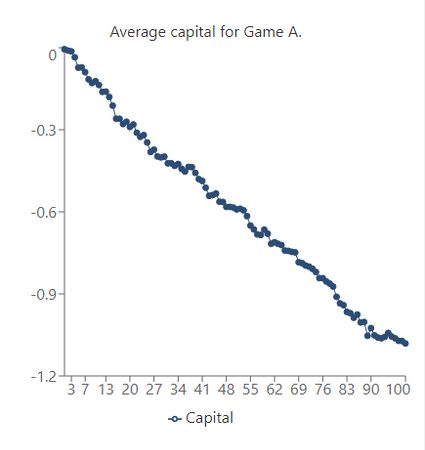
We can interpret this graph as a losing game. The more games we play, the further the graph will drop: we will lose money if we keep playing game A.

Game B

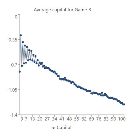
With the same downward trend in the graph, we can say that game B is also a losing game (but we already knew that).

AABB sequence

What if we play the sequence AABB (two games of A followed by two games of B)? What would our capital look like after playing 100 games following this pattern?

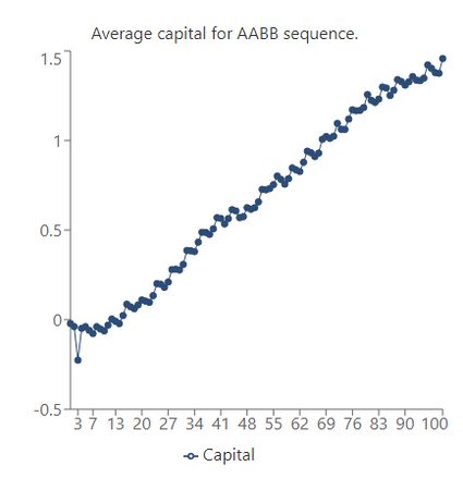
In this case, as the number of games goes up, the capital increases, too! This means that AABB is actually a winning strategy.

But why does this happen?

The short answer is that the AABB pattern allows the player to be in favorable states (more likely to win $1) more often than in unfavorable states (more likely to lose $1) of the system. So, even though each game has more unfavorable states, the combination AABB allows the player to play game B₂ (the winning game) more often.

If you're still not convinced, let's see how we can explain Parrondo's paradox using Markov chain analysis.

Markov chains can be used to model the transitions between different states of a system. In our example, they can be used to show how the probability of playing each game changes as the number of games increases.

We will use probability vectors $\pi$ (a column vector) and a matrix called the transition matrix $P$, which will simulate playing one game given a specific state:

Specifically,

• Each element $m_{ij}$ of $P$ represents the probability of transitioning from state $j$ to $i$.
• Each vector element $\pi_k^n$ is the probability of the system being at state $k$ after $n$ games.

Modelling game B

Let's say we want to model game B using this method.

To decide whether we play game B₁ or B₂ at a given time, we use the operation modulo 3 on our current capital (modulo delivers the remainder after dividing our capital by 3). So, no matter how many games we have played, this operation will return either 0, 1, or 2. We can separate our future capital into these three sets.

Since we have three possible states, our probability vector will have three components.

We can build the transition matrix for game B as follows:

Here each column corresponds to a state where the remainder of dividing our capital by 3 is 0, 1, or 2, respectively. And each element of said columns (from top to bottom) is the probability of transitioning to 0, 1, or 2, respectively.

If we're at state 2 (third column), for example, our capital is not a multiple of 3. Therefore we'll play game B₂:

• The probability of moving to state 0 is the probability of winning B₂ since our capital will then be a multiple of 3;
• The probability of moving to state 1 is the probability of losing B₂; and
• The probability of moving to state 2 is zero since we're at state 2, and we can only either lose or win.

Therefore, $P$ is equal to:

How to find the probability after a large number of games

These types of transition matrices involving probabilities are called stochastic, and there is a theorem called the Perron–Frobenius theorem, which ensures that the system will converge to a steady-state in the long run.

This means that after playing a large number of games, the probability of playing each of them doesn't change anymore:

Note that this is an eigenvalue equation for $\lambda = 1$.

If we apply this result to the transition matrix for game B, we can find the associated eigenvector and, therefore, the steady state.

You can use our eigenvalue and eigenvector calculator to verify that the eigenvector is:

We now divide each component by the sum of the components (since it's a probability vector) and obtain the steady state:

This means that by playing game B, we will be at state 0 (our capital is a modulus of 3, so we play the losing game) about %38.4 of the time.

To calculate the probability to win on game B, we just need to multiply the probability of being at each state by the probability of winning at each state and add them:

which proves that game B is a losing game.

Random sequence

We can apply the same analysis to a random pick between games A and B.

If we toss a fair coin to decide which game to play (50/50 odds), the transition matrix is:

The resulting steady-state vector is:

This gives us a winning probability of:

This shows that even if we play both losing games (A and B) in a random sequence, we are guaranteed to win in the long run!

This setup is not the only scenario where Parrondo's paradox appears. By making the probabilities of winning each game differ by ε (linking them), one can prove that the paradox emerges in other combinations of games and conditions as long as ε is sufficiently small.

To replicate the paradox by yourself, you should:

1. Pick a small value ε (ε < 0.005) to make the probabilities of each game differ slightly.
2. Write the probabilities of each game:
   • Win game A = 0.5 - ε;
   • Win game B₁ (played if capital is multiple of 3) = 0.1 - ε;
   • Win game B₂ (played if capital is not a multiple of 3) = 0.75 - ε.
3. Pick an order or sequence to alternate between games A and B.
4. Repeat several times and average the capital after a set number of games.

No. Parrondo's paradox only works in specific scenarios where games A and B are related by an external mean — in the simplest case, the player's capital.

No. Parrondo's paradox can emerge in any game where a relation exists between the games to be played. Games such as dice-tossing or other random processes can also exhibit the behavior of this paradox.