Exponential Growth Calculator

There is a substantial number of processes for which you can use this exponential growth calculator. The general rule of thumb is that the exponential growth formula:

is used when there is a quantity with an initial value, $x_0$, that changes over time, $t$, with a constant rate of change, $r$. The exponential function appearing in the above formula has a base equal to $1 + r/100$.

Note that the exponential growth rate, $r$, can be any positive number, but this calculator also works as an exponential decay calculator — where $r$ also represents the rate of decay, which should be between 0 & -100%. The reason for this is that you cannot have a decline of more than 100% with regard to the initial quantity, as it would result in a negative value.

The exponential growth equation is used in radiocarbon dating, PCR (you can discover why with our annealing temperature calculator), as well as in calculating compound interest. To learn more, please see our compound interest calculator. For more examples of where you can use this formula, please check below.

Consider the following problem: the population of a small city at the beginning of 2019 was 10,000 people. It was noticed that the population of the city grows at a steady rate of 5% annually. What should you do to calculate the projected population size in the year 2030? From the given data, we can conclude the initial population value, $x_0$, equals 10,000. Also, we have a growth rate of $r = 5\%$

Therefore, the exponential growth formula we should use is:

Here $t$ is the number of years passed since 2019. In our case, for the year 2030, we should use $t = 11$, since this is the difference in the number of years between 2030 and the initial year 2019. Finally, we get:

So, the projected number of inhabitants of our small city in the year 2030 is around 17,103.

If you want to dig a bit deeper into this particular formula, you can use our exponential growth calculator to find out the projected number of inhabitants for each year, starting from 2019. This calculation results in the following table, where we round the results to the nearest integer:

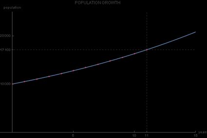
If you want to get an even better feel for the population growth, you may represent this data graphically, with the horizontal axis being the time axis and the vertical axis representing the population value $x(t)$. The data from the table are all points lying on the continuous graph of the exponential growth function:

Since the base of this exponential function is 1.05, and since it is greater than 1, the exponential growth graph we get is rising. The main difference between this graph and the normal exponential function graph is that its y-intercept is not 1 but 10,000, which corresponds to the initial value $x_0$:

From this example, we can see the possible limitations of the exponential growth model — it is unrealistic for the rate of growth to remain constant over time. Namely, it is hard to expect that the yearly rate of growth for the city's population would remain at 5% for a decade or more.

In real-life situations, there are natural oscillations of the rate of growth that are not included in this model of exponential growth. A more realistic model of population growth is the logistic growth model, which has the carrying capacity, a constant representing the population's natural growth limit.

Continuing with our small city, the next question you may ask yourself is, "when can we expect the population to reach some important value?" This is useful if you want to know when to adjust the city's urban planning for a larger population, so the city council needs to know which year they can expect the city's population to have tripled in size from the original 10,000?

Here, we know how much is $x(t)$, but we don't know the value of t when this will happen. Let's do it step by step:

1. Insert $x(t) = 30,\!000$ into the formula: $30,\!000 = 10,\!000 \cdot 1.05^{t}$

2. After dividing both sides of the equation by 10,000, we get: $1.05^{t} = 3$.

3. Take the logarithm to the base 1.05 of both sides of this equation: $t = \log_{1.05} 3$.

4. Use the logarithm to finally get: $t = 22.52$.

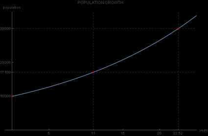
So, the answer to the council's question is approximately 22 years after the initial year of 2019, so in 2041:

You may have already noticed a problem with exponential growth and decay, that it naturally treats time as only a positive value, so we are predicting a future quantity. However, this does not prevent us from using this formula with negative time values. This means that we describe the phenomenon of interest in the time before the initial observation was made.

In the case of population growth, you may ask the question: what was the population of our small city in the year 2000, assuming the population growth rate was a constant 5%?

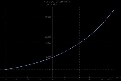
To solve this, you would use $t = -19$ since the year 2000 precedes the year 2019 by 19 years. The answer would therefore be:

inhabitants, as you can also see on this graph:

For some applications, for example when calculating the exponential decay of a radioactive substance, an alternative way of writing down the formula for exponential growth and decay is more productive:

The coefficient $k$ plays the role of the rate of growth, similarly as r does in the original exponential growth formula. Comparing the above equation with the original one, you can see that the relation between $r$ and $k$ is as follows:

which means $r = 100 \cdot (e^k- 1)$ and $k = \ln(1 + r/100)$.

Radioactive decay is a well-known example of where the exponential decay formula is used. For a given initial quantity of radioactive substance, you may write down the law which governs its decay over time. But, maybe a more fun example is to measure how much coffee remains in your body at 10 pm if you drank a cup of coffee with $x_0 = 95\ \rm mg$ of caffeine at noon.

We will use the fact that the half-life of caffeine in the human body is approximately six hours. Half-life is defined as the time needed a given quantity to reduce to half of its initial value. So, in this example we have

$x(6) = 1/2 \cdot 95 \text{ mg} = 47.5 \text{ mg}$

Here, it will be easier to use the alternative notation for the exponential growth formula:

$x(t) = 95 \cdot e^{kt}$

Here is the step-by-step calculation:

1. Insert x(6)= 47.5 and t = 6 into the equation: $47.5 = 95 \cdot e^{6k}$.

2. This expression, after dividing both sides of the equation by 95 and applying the natural logarithm, gives: $6\cdot k = \ln 0.5$.

3. By using the natural logarithm, we get: $k = -0.1155$.

4. Therefore, the exponential decay formula in our example is: $x(t) = 95 \cdot e^{-0.1155 \cdot t}$.

5. Since 10 pm is ten hours later than noon, we want to know the amount of caffeine at $t = 10$. We have: $x(10) = 95 \cdot e^{-0.1155 \cdot 10} = 29.9305$.

So, at 10 pm, the amount of caffeine remaining in your body will be approximately 30 mg.

Time can be expressed in basically any appropriate units. For some problems, these will be seconds, for others, years. You should choose the time unit in a way that corresponds to the nature of the observed process. For example, if you want to understand the change in the population of a city, you should choose years. On the other hand, if you're going to calculate the amount of coffee remaining in your body after you drank a cup of it, the appropriate time unit should be hours or maybe minutes.

Please note that $t$ doesn't really have to be considered as time only. In some cases, the variable which measures the rate of change can be different than time. For example, when studying the way that atmospheric pressure changes with altitude, the variable measuring this change is distance, and you should choose meters as the appropriate units of change. Our Air pressure at altitude calculator can help here.

The difference in the exponential growth rate r will have a significant influence on how quickly the observed quantity changes from the initial value. Let us start with $x_0 = 100$ and, using the exponential growth calculator, see what $x(10)$ will be for four different values of $r$:

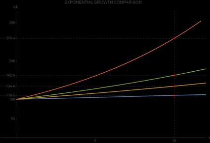
From this table, we see that all initial values are the same, being equal to $x_0 = 100$, but the final values of $x(10)$ differ significantly. Your intuition may trick you here because the difference between 1% and 3% doesn't look like much, but after ten periods, this amounts to a 21.67% higher value for $x(10)$ for 3%-growth as compared to 1%-growth.

If you compare the 10%-growth to 5%-growth, you will notice an even greater difference, 59.23%, in favor of 10%-growth. You can observe this contrast in the following graphical representation of the four exponential growth functions:

The formula for exponential growth and decay is used to model various real-world phenomena:

• Population growth of bacteria, viruses, plants, animals, and people;
• Decay of radioactive matter;
• Blood concentration of drugs;
• Atmospheric pressure of air at a certain height;
• Compound interest and economic growth;
• Radiocarbon dating; and
• Processing power of computers etc.

How Populations Grow: The Exponential and Logistic Equations

Two Models of Population Growth

The World’s Population Hasn’t Grown Exponentially for at Least Half a Century

Exponential Population Growth

Caffeine Pharmacology

Caffeine Effects on Sleep Taken 0, 3, or 6 Hours before Going to Bed