Phillips Curve Calculator

By applying the Phillips curve calculator, you can study the relationship between inflation and other Phillips curve model variables. Since the Phillips curve went through considerable development due to the continuous development of macroeconomic theories, we included the following three versions of the Philips curve in the Phillips curve equation calculator :

• Traditional Phillips curve;
• New classical Phillips curve; and
• New Keynesian Phillips curve (NKPC).

Each of these options reflects a different theoretical economic background. Read further and learn the Phillips curve definition and the difference between the short-run and long-run Phillips curve in economics. We will also show you the short-run Phillips curve graph and explain what the expectations augmented Phillips curve is.

The concept of the Phillips curve comes from a famous 1958 paper by the New Zealand–born economist A. William Phillips. Studying the historical data for Britain, he found that when the unemployment rate was high, the wage rate was falling, and when the unemployment rate was low, the wage rate was rising.

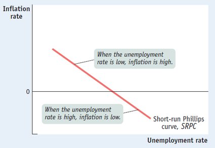
Other economists soon found a similar relationship between the unemployment rate and inflation in other industrialized economies. The conclusion became clear: there is a negative short-run relationship between the unemployment rate and the inflation rate, which can be plotted as a short-run Phillips curve.

This short-term trade-off between unemployment and inflation is represented in the below short-run Phillips curve graph: lower unemployment leads to higher inflation, and vice versa.

The initial form of the Phillips curve, à la Phillips, describes the empirical phenomena where the unemployment rate drives the growth rate of money wages. Therefore, this basic Phillips curve shows the relationship between money wages and the unemployment rate.

The traditional Phillips curve is the simplest one we included in the Phillips curve calculator and in its original form as outlined by Phillips himself.

This Phillips curve equation says that the rate of growth of the money wage rate depends on the trend rate of growth of money wages and the unemployment rate. This can be written in the following form:

where:

• The operator $g$ – The percentage rate of growth of the variable that follows;
• $W$ – Money wage rate representing the total money wage costs per production employee, including benefits and payroll taxes;
• $W^T$ – Trend rate of growth of money wages; and
• $f(U)$ – Unemployment rate in a given function.

In other words, periods of above-average inflation tend to be associated with above-trend economic activity (i.e., higher than expected GDP growth rate), for example, as measured by a relatively low unemployment rate.

Parallel with the progression of economic theories, economists became more interested in finding theoretical foundation for the Phillips curve equation. It led to the appearance of the New Classical Phillips curve, which is derived from a classical economic model following simple economic principles.

More precisely, it is the Lucas aggregate supply function augmented by the concept of the natural rate of unemployment (or NAIRU) and the Okun's law which drives to the final form of the New Classical Phillips curve that we use in the Phillips curve calculator:

where:

• $b$ – Positive constant;
• $U$ – Unemployment rate;
• $U_n$ – Natural rate of unemployment, or NAIRU; and
• $v$ – Unexpected exogenous supply shocks.

The New Keynesian Phillips curve (NKPC), first introduced in 1995, constitutes one of the key building blocks for the New Keynesian general equilibrium model. Due to the high complexity of the model and the limited space here, we'll introduce only its main features and parameters. If you'd like a deeper insight into this topic, feel free to take a look at the article titled The New Keynesian Phillips Curve: Lessons From Single-Equation Econometric Estimation. You can also use our Phillips curve calculator without fully understanding the math behind it!

The NKPC is a structural model of inflation dynamics where one of the key driving factors is price stickiness, the parameter that governs the passthrough of marginal costs into inflation. In other words, the NKPC model takes into consideration the fact that firms do not update the prices of their products constantly and uniformly; instead, they keep their prices fixed over a specific interval. Therefore, prices do not reflect the actual condition of the economy immediately. The average price duration provides a measure of the degree of price stickiness. The higher the parameter (the stickier the prices), the more limited the transition of marginal costs into inflation, making the Phillips curve flatter.

The Phillips curve equation calculator uses the following sets of equations to describe the New Keynesian Phillips curve model:

where:

• $\pi_{t+1}$ – Inflation rate at period $t+1$;

• $E_t\{\pi_{t+1}\}$ – Inflation expectation at period $t$;

• $\tilde{y}_t$ – Output gap: the difference between the actual output and its potential level at period $t$ – learn more about it at our GDP gap calculator;

• $\beta$ – Households’ discount factor (the default value of 0.99 implies a steady state real return on financial assets of about 4 percent);

• $\theta$ – Price stickiness: This parameter represents the average time over which prices are kept fixed (the default value of 0.75 implies an average price duration of four quarters);

• $\sigma$ – Utility of consumption: intertemporal elasticity of substitution;

• $\varphi$ – Disutility of labor: the inverse labor supply elasticity (the default value of 5 implies a Frisch elasticity of labor supply of 0.2);

• $\alpha$ – Labor supply elasticity;

• $\epsilon$ – Demand elasticity: a measure of the change in the quantity of a product purchased in relation to a change in its price (the default value of 9 implies a steady state markup value of 12.5 percent);

• $\bar y_t$ – Potential output: a hypothetical level of output associated with flexible prices in the economy at period $t$; and

• $y_t$ – Actual output or GDP at period $t$.

The Phillips curve represents the inverse relationship between inflation and unemployment.

In its modern form, it is a relationship between inflation, cyclical unemployment, expected inflation, and supply shocks derived from the short-run aggregate supply curve.

The natural rate of unemployment corresponds to the number of unemployed people due to structural issues in the labor market caused by new technology or lack of skills required to gain employment.

NAIRU (non-accelerating inflation rate of unemployment) is the particular level of unemployment associated with an economic condition resulting in stable inflation.

While multiple versions of the Phillips curve exist, they all have one common point: they all take inflation into account.

However, they might not include inflation in the same way during the calculation procedure.

The Phillips curve shows the relationship between inflation and unemployment. While inflation and unemployment are inversely related in the short run, there is no trade-off in the long run.

There are three common forms of Phillips curves in economics:

1. Traditional Phillips curve, which is the original form where the unemployment rate drives the growth rate of money wages;
2. New classical Phillips curve, which follows economical principles based on the classical theoretical model; and
3. New Keynesian Phillips curve (NKPC), which is the key building block for the most advanced New Keynesian general equilibrium models.