Wilcoxon Rank-Sum Test Calculator
Welcome to Omni's Wilcoxon rank-sum test calculator! This calculator can perform both the exact Wilcoxon rank-sum test and use a normal approximation as well! Scroll down to learn all things related to the beloved Wilcoxon rank-sum test, a.k.a. the Wilcoxon-Mann-Whitney test.
Wondering what the Wilcoxon rank-sum test is? Not sure how to interpret the Wilcoxon rank-sum test? We will give you the Wilcoxon rank-sum test formula along with a step-by-step explanation of how to calculate the Wilcoxon rank-sum test. Once the basics are clear, we dive into the question of when to use the Wilcoxon rank-sum test and discuss the interpretation of the Wilcoxon rank-sum test. As a bonus, we'll explain the difference between Wilcoxon rank-sum and signed-rank tests.
Keep in mind that this Wilcoxon rank-sum test calculator uses the sum of ranks as the test statistic. For the well-known U statistic, see our dedicated Mann-Whitney U test calculator.
What is the Wilcoxon rank-sum test?
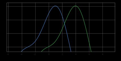
The Wilcoxon rank-sum test is a statistical test that can help you decide whether two samples come from the same distribution or from different (shifted) distributions. If so, then you can deduce if the two populations have the same or different medians. For instance, in the picture below, there are two distributions (more precisely, their probability density functions) that would be identical if not for the shift. As we can see, the green distribution is shifted to the right with respect to the blue one. As a result, the median of the green distribution is greater than the median of the blue one.
💡 The Wilcoxon rank-sum test is sometimes called the Wilcoxon-Mann-Whitney test or a Mann-Whitney U-test, as it was proposed by Wilcoxon and further developed by Mann and Whitney. However, this development led to a slightly different version of the test, equivalent to the original one. The final decision is always the same, but the calculations are slightly different.
Now that we know what the Wilcoxon rank-sum test is all about, it's time we discuss when you should use this test.
When to use the Wilcoxon rank-sum test?
Have you already heard of the two-sample t-test, the default choice when we want to test if the population means for two independent samples are equal or not? If not, you discover it with our dedicated t-test calculator. Wilcoxon rank-sum test has a similar purpose, but it has fewer assumptions than the t-test.
Namely, as you may recall, in the t-test, either each sample has to follow the normal distribution or the samples have to be sufficiently large (a rule of thumb: more than 30 elements each). The latter condition allows us to make use of the central limit theorem.
In consequence, if your sample is not normally distributed (e.g., it is skewed) and it has relatively few elements, then the t-test is not for you. And that's when the Wilcoxon rank-sum test triumphantly enters the stage!
Having discussed the question of when to use the Wilcoxon rank-sum test, we now move on to the problem of the interpretation of the Wilcoxon rank-sum test.
How do I interpret Wilcoxon rank-sum test?
The null hypothesis of the Wilcoxon test is that the two populations, say A and B, have the same distribution. If we reject the null, that means we have evidence that the distributions are shifted with respect to each other. The three possible alternative hypotheses are the following:
-
A > B: distribution of A is shifted to the right with respect to the distribution of B.
-
A < B: distribution of A is shifted to the left with respect to the distribution of B.
-
A ≠ B: distribution of A is shifted to the right or to the left with respect to the distribution of B.
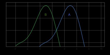
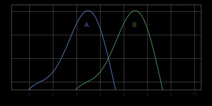
In the pictures below you can see the hypothesis A > B (upper figure) and the hypothesis A < B (bottom figure):
Clearly, under the null hypothesis, the two populations have equal medians, and so rejecting the null means that we have evidence that the medians are different. In terms of medians, the three possible alternative hypotheses are the following:
-
Median of population A > median of population B;
-
Median of population A < median of population B; and
-
Median of population A ≠ median of population B.
We perform a one-sided test if there is a prior theory leading us to believe that one population has a distribution shifted to the right/left as compared to the other population. Otherwise, we perform a two-sided test.
How do I use this Wilcoxon rank-sum test calculator?
- Input your data into the dedicated fields. The more observations you enter, the more fields will appear. The maximum is 50 observations in each sample.
- Set up the test – choose the significance level and the alternative hypothesis.
- The results of the Wilcoxon rank-sum test appear immediately at the bottom of the calculator.
- If the calculator approximates the distribution of the test statistic with a normal distribution, then you can choose between the p-value approach and critical region approach:
- If both samples have fewer than
20elements, then the calculator performs the exact Wilcoxon rank-sum test, i.e., it uses the exact distribution of the test statistic. You can force it to use the normal distribution by setting theUse normal approximationoption toYes. - If at least one of the samples has more than
20elements, the calculator uses the normal approximation by default.
- If both samples have fewer than
- In the
Advanced modeof the calculator, you can decide whether to use the corrections for ties and continuity. See the last section for an explanation.
Should you ever need to perform this test by hand, in what follows, we will not only show you the Wilcoxon rank-sum test formula but also explain step-by-step how to calculate the Wilcoxon rank-sum test!
How do I calculate Wilcoxon rank-sum test?
To perform the Wilcoxon rank-sum test, you have to:
- Rank from lowest to highest the observations in the two samples combined.
- Compute the test statistics — it's the sum of ranks in one of the samples.
- If your samples are small, perform the exact Wilcoxon rank-sum test: compare the test statistic with critical values for the Wilcoxon rank-sum test (to be found in statistical tables), taking into account the alternative hypothesis.
- Otherwise, use the normal approximation and make a decision based on the critical values or the p-value.
In what follows, we unpack these instructions. Let us introduce some necessary notation. By n₁ and n₂, we will denote the number of observations in Sample A and Sample B, respectively, and n will stand for the total number of observations, i.e., n = n₁ + n₂.
Ranking the observations
Take values from the entire data set, i.e., from Sample A and Sample B combined, and order them from lowest to highest. The lowest observation receives rank 1, the second-lowest receives rank 2, and so on, all the way up to the highest observation, which receives rank n.
This is very simple; you only need to be a bit more careful when there are ties – that is, if the same value appears in the data set a few times. In such a case, you should assign the same rank to all the identical observations. This rank is equal to the arithmetic mean of the consecutive ranks you would assign to these observations if they were all different.
That is, assume the last rank we used is p, and now we see that some observation appears k times in the data set. The consecutive ranks we would use are p+1, p+2, ..., p+k. We calculate their arithmetic mean, i.e., (p+1 + p+2 + ... + p+k) / k, and assign this value as the common rank of our k identical entries. It may happen that this rank is not an integer, but this is not a problem!
Computing the test statistics
The test statistic in the Wilcoxon rank-sum test is the sum of the ranks for either of the two samples. We will pick the sum of ranks in Sample A and denote it by R₁.
In fact, the sum of ranks in one sample fully determines the sum of ranks in the other sample. To see this, denote by R₂ the sum of ranks in Sample B. Clearly, the sum of all ranks is equal to R₁ + R₂. On the other hand, the sum of all ranks is equal to the sum of all consecutive numbers between 1 and n, which is n(n + 1)/2. Hence, we have the following relationship:
R₂ = n(n + 1)/2 - R₁.
We observe that the test statistic R₁ has a discrete distribution, its minimal possible value is n₁(n₁ + 1)/2, and its maximal possible value is n₁(n₁ + 2n₂ + 1)/2. Indeed, R₁ takes the smallest possible value when every observation from Sample A is smaller than (or equal to) every observation from Sample B. So Sample A receives the lowest ranks, i.e., 1, ..., n₁. On the other hand, R₁ takes the highest possible value when every observation from Sample A is greater than (or equal to) every observation from Sample B. So Sample A receives the highest possible ranks, i.e., n₂ + 1, ..., n₂ + n₁.
Critical values for the Wilcoxon rank-sum test
The critical value and the direction of comparison (> or <) depends on the alternative hypothesis you've chosen. As we remember, there are three possibilities:
-
A > B: distribution of A is shifted to the right with respect to the distribution of B.
If A > B, then the observations from Sample A tend to have greater ranks than those from Sample B. Hence, we have evidence in favor of the alternative if R₁ is unusually large. In other words, testing against the alternative A > B, we would reject H₀ for large values of R₁. Consequently, the critical region is right-sided, i.e., of the form [c, ∞), where c is the critical value.
-
A < B: distribution of A is shifted to the left with respect to the distribution of B.
If A < B, then the observations from Sample A tend to have lower ranks than those from Sample B. Hence, we have evidence in favor of this alternative if c R₁ is unusually small. In other words, testing against the alternative A < B, we would reject H₀ for small values of R₁. Consequently, the critical region is left-sided, i.e., of the form (-∞, c], where c is the critical value.
-
A ≠ B: distribution of A is shifted to the right or to the left with respect to the distribution of B.
We have evidence in favor of this alternative if R₁ is extreme, i.e., unusually small or unusually large. This means that the critical region is two-sided, i.e., of the form (-∞, c₁] ∪ [c₂, ∞), where c₁ and c₂ are the critical values. Actually, taking into account the minimal and maximal possible values of R₁, we can rewrite the critical region as [n₁(n₁ + 1)/2, c₁] ∪ [c₂, n₁(n₁ + 2n₂ + 1)/2].
If you want to perform the exact Wilcoxon rank-sum test, you have to use the critical values based on the actual distribution of R₁. In such a case, the critical values c, c₁, c₂ depend on both n₁ and n₂ and the significance level. OK, but how do I determine these values, you may (and should) ask. Well, you have to use either a statistical package or the tables of the distribution of the sum of ranks, which you can find in a book or online. Another (and much simpler) way is to use our Wilcoxon rank-sum test calculator!
Resorting to the normal approximation
If your sample is large enough (as few as 5 observations in each sample is enough, but the more, the better), then you can successfully approximate the distribution of R₁ with the normal distribution with the following parameters:
-
mean: μ = n₁(n₁ + n₂ + 1) / 2;
-
variance: σ² = n₁n₂(n₁ + n₂ + 1) / 12.
In practice, we use the normalized test statistic:
z = (R₁ − μ) / σ
to get the z-score and compare it with the quantiles of the standard normal distribution N(0,1) to get the p-value. If you're not yet familiar with the p-value approach to hypothesis testing, check out Omni's p-value calculator.
And that's it when it comes to the question of how to calculate the Wilcoxon rank-sum test! One more detail is worth mentioning, namely that of corrections for ties and continuity.
Corrections for ties and continuity
In this final section, we discuss the corrections for ties and continuity that are available in Omni's Wilcoxon rank-sum test calculator:
-
Ties correction
The presence of ties slightly disturbs the default (above-mentioned) normal approximation of the distribution of R₁. What the researchers often do is apply a slightly different formula for variance:
σ² = n₁n₂(n₁ + n₂ + 1)(1 − Cₜ) / 12
where Cₜ is the correction for ties defined as:
Ct = ∑j (rj³ − rj) / (n³ − n)
where rj is the number of times (i.e., frequency) the rank j appears, with j varying over the set of tied ranks (or, equivalently, over the set of all ranks).
Clearly, if there are no ties, then Ct = 0, and the formula for σ² goes back to its default form.
-
Continuity correction
When we approximate the distribution of R₁ (which is a discrete distribution) with a normal distribution (which is a continuous distribution), we often apply a continuity correction. We do this by slightly changing the formula for the z-score. Actually, the exact formula of this correction depends on the alternative hypothesis:
-
A > B:
z = (R₁ − μ − 0.5) / σ
-
A < B:
z = (R₁ − μ + 0.5) / σ
-
A ≠ B:
z = (R₁ − μ − 0.5) / σ, if R₁ ≥ μ
z = (R₁ − μ + 0.5) / σ, if R₁ < μ
-
FAQ
What is the difference between the Wilcoxon rank-sum and signed-rank tests?
The Wilcoxon rank-sum test and signed-rank tests are non-parametric alternatives to the two-sample t-test and paired t-test, respectively:
- Use the Wilcoxon rank-sum test to compare two independent samples.
- Use the Wilcoxon signed-rank test to compare the results of repeated measurements on a single sample.
What is the difference between the Wilcoxon rank-sum and Mann-Whitney U tests?
The Wilcoxon rank-sum and Mann-Whitney U tests are the same test and they always lead you to the same decision regarding your data. They use test statistics that may appear different at first sight, but, in fact, always produce the same result. The U statistic is used more often as it is not influenced by the sample size, as is the case with the sum of ranks statistics.